Note
Click here to download the full example code
Plotting vectors
Plotting vectors is handled by pygmt.Figure.plot.
import numpy as np
import pygmt
Plot Cartesian Vectors
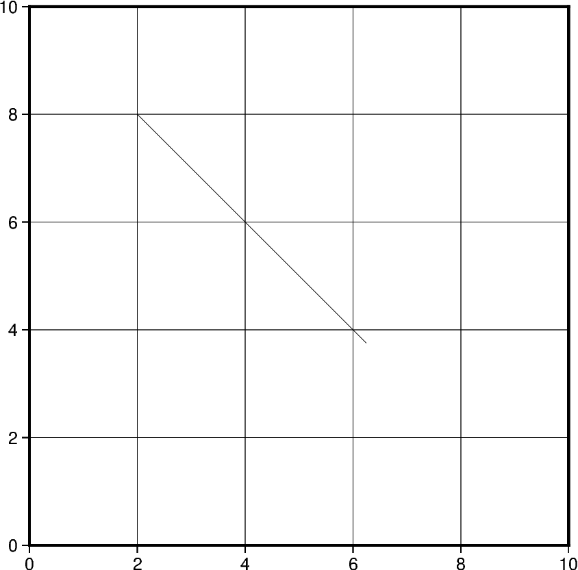
Create a simple Cartesian vector using a starting point through
x, y, and direction parameters.
On the shown figure, the plot is projected on a 10cm X 10cm region,
which is specified by the projection parameter.
The direction is specified
by a list of two 1d arrays structured as [[angle_in_degrees], [length]].
The angle is measured in degrees and moves counter-clockwise from the
horizontal.
The length of the vector uses centimeters by default but
could be changed using pygmt.config
(Check the next examples for unit changes).
Notice that the v in the style parameter stands for
vector; it distinguishes it from regular lines and allows for
different customization. 0c is used to specify the size
of the arrow head which explains why there is no arrow on either
side of the vector.
Out:
<IPython.core.display.Image object>
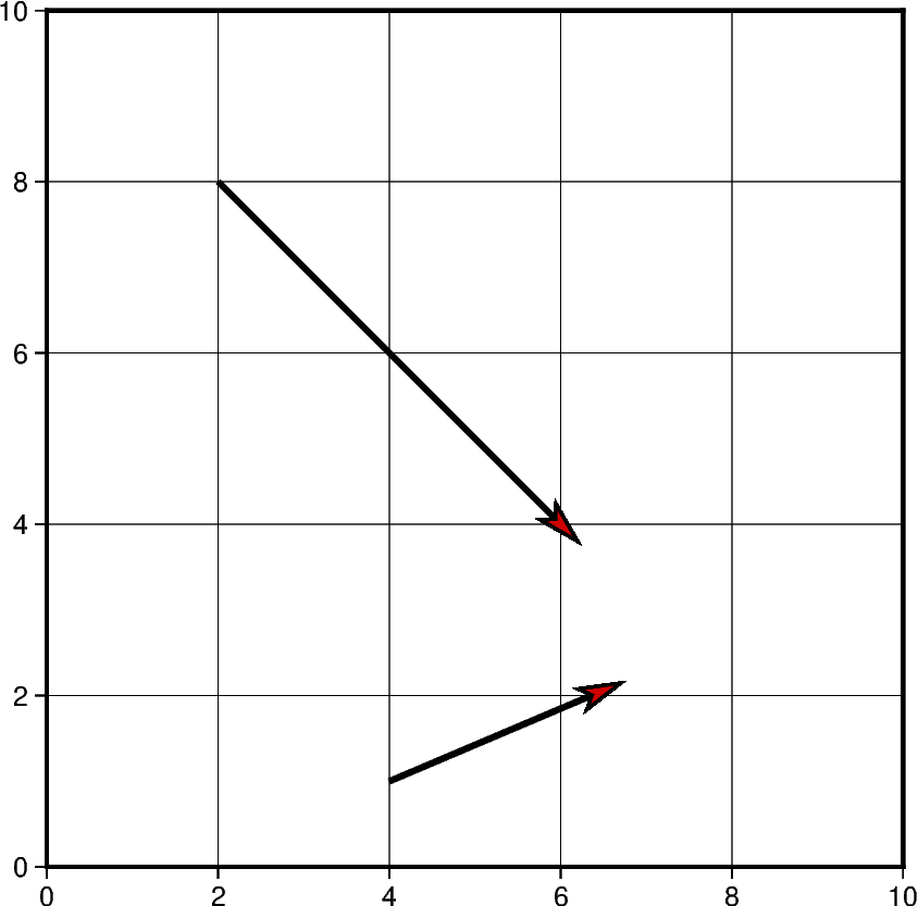
In this example, we apply the same concept shown previously to plot multiple
vectors. Notice that instead of passing int/float to x and y, a list
of all x and y coordinates will be passed. Similarly, the length of direction
list will increase accordingly.
Additionally, we change the style of the vector to include a red
arrow head at the end (+e) of the vector and increase the
thickness (pen="2p") of the vector stem. A list of different
styling attributes can be found in
Vector heads and tails.
Out:
<IPython.core.display.Image object>
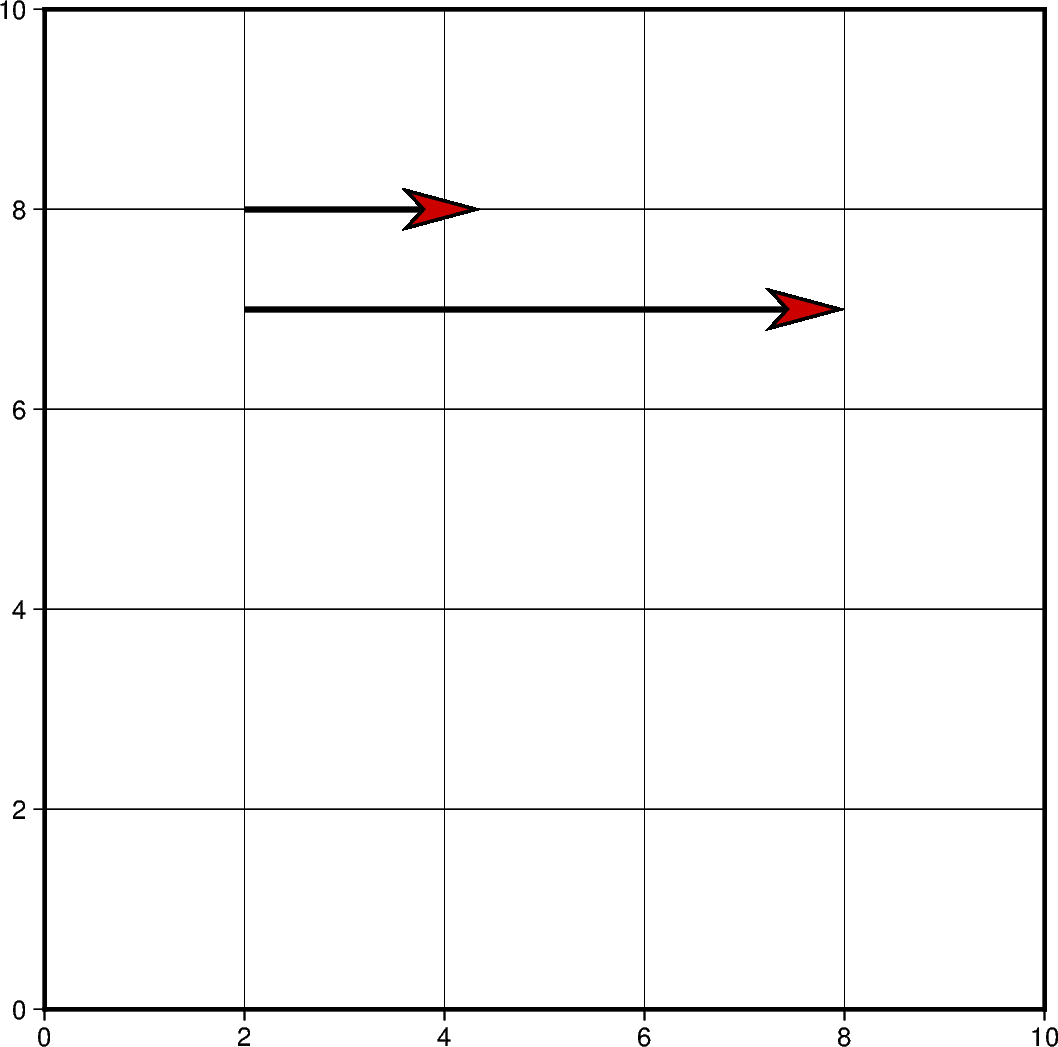
The default unit of vector length is centimeters, however, this can be changed to inches or points. Note that, in PyGMT, one point is defined as 1/72 inch.
In this example, the graphed region is 5in X 5in, but
the length of the first vector is still graphed in centimeters.
Using pygmt.config(PROJ_LENGTH_UNIT="i"), the default unit
can be changed to inches in the second plotted vector.
fig = pygmt.Figure()
# Vector 1 with default unit as cm
fig.plot(
    region=[0, 10, 0, 10],
    projection="X5i/5i",
    frame="ag",
    x=2,
    y=8,
    style="v1c+e",
    direction=[[0], [3]],
    pen="2p",
    color="red3",
)
# Vector 2 after changing default unit to inch
with pygmt.config(PROJ_LENGTH_UNIT="i"):
    fig.plot(
        x=2,
        y=7,
        direction=[[0], [3]],
        style="v1c+e",
        pen="2p",
        color="red3",
    )
fig.show()
Out:
<IPython.core.display.Image object>
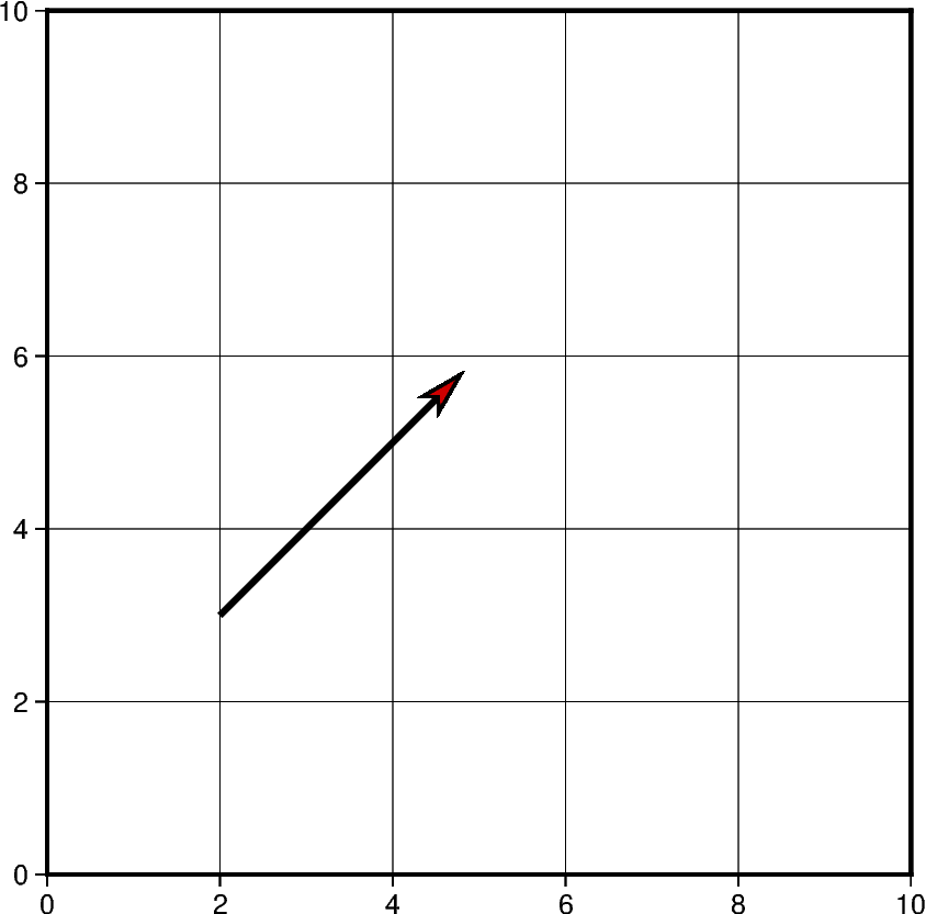
Vectors can also be plotted by including all the information
about a vector in a single list. However, this requires creating
a 2D list or numpy array containing all vectors.
Each vector list contains the information structured as:
[x_start, y_start, direction_degrees, length].
If this approach is chosen, the data parameter must be
used instead of x, y and direction.
Out:
<IPython.core.display.Image object>
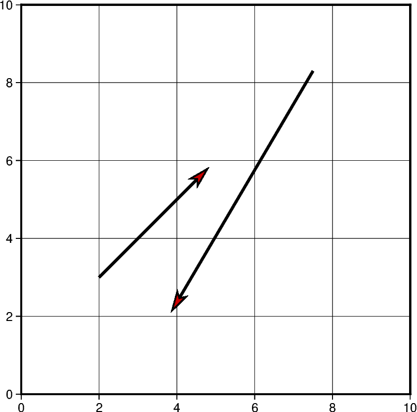
Using the functionality mentioned in the previous example,
multiple vectors can be plotted at the same time. Another
vector could be simply added to the 2D list or numpy
array object and passed using data parameter.
# Vector specifications structured as:
# [x_start, y_start, direction_degrees, length]
vector_1 = [2, 3, 45, 4]
vector_2 = [7.5, 8.3, -120.5, 7.2]
# Create a list of lists that include each vector information
vectors = [vector_1, vector_2]
# Vectors structure: [[2, 3, 45, 4], [7.5, 8.3, -120.5, 7.2]]

fig = pygmt.Figure()
fig.plot(
    region=[0, 10, 0, 10],
    projection="X10c/10c",
    frame="ag",
    data=vectors,
    style="v0.6c+e",
    pen="2p",
    color="red3",
)
fig.show()
Out:
<IPython.core.display.Image object>
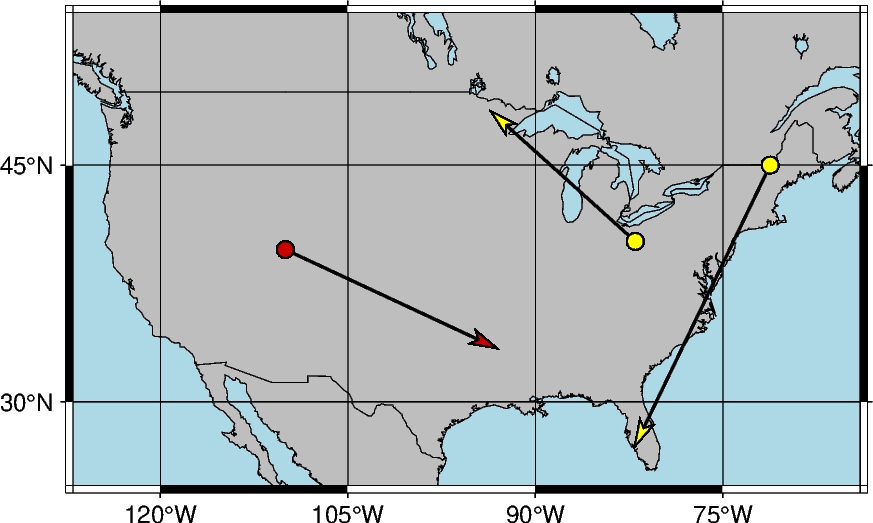
In this example, cartesian vectors are plotted over a Mercator projection of the continental US. The x values represent the longitude and y values represent the latitude where the vector starts.
This example also shows some of the styles a vector supports. The beginning point of the vector (+b) should take the shape of a circle (c). Similarly, the end point of the vector (+e) should have an arrow shape (a) (to draw a plain arrow, use A instead). Lastly, the +a specifies the angle of the vector head apex (30 degrees in this example).
# Create a plot with coast, Mercator projection (M) over the continental US
fig = pygmt.Figure()
fig.coast(
    region=[-127, -64, 24, 53],
    projection="M10c",
    frame="ag",
    borders=1,
    shorelines="0.25p,black",
    area_thresh=4000,
    land="grey",
    water="lightblue",
)

# Plot a vector using the x, y, direction parameters
style = "v0.4c+bc+ea+a30"
fig.plot(
    x=-110,
    y=40,
    style=style,
    direction=[[-25], [3]],
    pen="1p",
    color="red3",
)

# vector specifications structured as:
# [x_start, y_start, direction_degrees, length]
vector_2 = [-82, 40.5, 138, 2.5]
vector_3 = [-71.2, 45, -115.7, 4]
# Create a list of lists that include each vector information
vectors = [vector_2, vector_3]

# Plot vectors using the data parameter.
fig.plot(
    data=vectors,
    style=style,
    pen="1p",
    color="yellow",
)
fig.show()
Out:
<IPython.core.display.Image object>
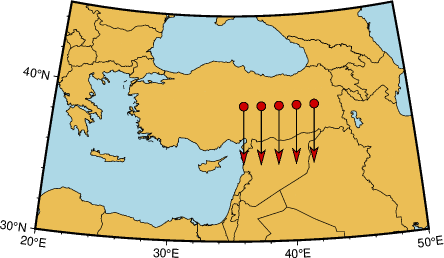
Another example of plotting cartesian vectors over a coast plot. This time a
Transverse Mercator projection is used. Additionally, numpy.linspace
is used to create 5 vectors with equal stops.
x = np.linspace(36, 42, 5)  # x values = [36.  37.5 39.  40.5 42. ]
y = np.linspace(39, 39, 5)  # y values = [39. 39. 39. 39.]
direction = np.linspace(-90, -90, 5)  # direction values = [-90. -90. -90. -90.]
length = np.linspace(1.5, 1.5, 5)  # length values = [1.5 1.5 1.5 1.5]

# Create a plot with coast, Mercator projection (M) over the continental US
fig = pygmt.Figure()
fig.coast(
    region=[20, 50, 30, 45],
    projection="T35/10c",
    frame=True,
    borders=1,
    shorelines="0.25p,black",
    area_thresh=4000,
    land="lightbrown",
    water="lightblue",
)

fig.plot(
    x=x,
    y=y,
    style="v0.4c+ea+bc",
    direction=[direction, length],
    pen="0.6p",
    color="red3",
)

fig.show()
Out:
<IPython.core.display.Image object>
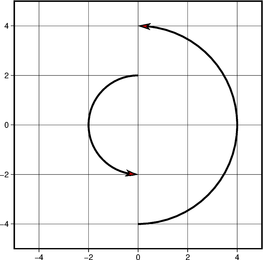
Plot Circular Vectors
When plotting circular vectors, all of the information for a single vector is
to be stored in a list. Each circular vector list is structured as:
[x_start, y_start, radius, degree_start, degree_stop]. The first two
values in the vector list represent the origin of the circle that will be
plotted. The next value is the radius which is represented on the plot in cm.
The last two values in the vector list represent the degree at which the plot
will start and stop. These values are measured counter-clockwise from the
horizontal axis. In this example, the result show is the left half of a
circle as the plot starts at 90 degrees and goes until 270. Notice that the
m in the style parameter stands for circular vectors.
fig = pygmt.Figure()

circular_vector_1 = [0, 0, 2, 90, 270]
data = [circular_vector_1]
fig.plot(
    region=[-5, 5, -5, 5],
    projection="X10c",
    frame="ag",
    data=data,
    style="m0.5c+ea",
    pen="2p",
    color="red3",
)

# Another example using np.array()
circular_vector_2 = [0, 0, 4, -90, 90]
data = np.array([circular_vector_2])

fig.plot(
    data=data,
    style="m0.5c+ea",
    pen="2p",
    color="red3",
)
fig.show()
Out:
<IPython.core.display.Image object>
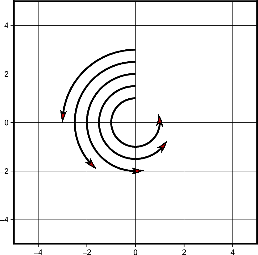
When plotting multiple circular vectors, a two dimensional array or numpy
array object should be passed as the data parameter. In this example,
numpy.column_stack is used to generate this two dimensional array.
Other numpy objects are used to generate linear values for the radius
parameter and random values for the degree_stop parameter discussed in
the previous example. This is the reason in which each vector has a different
appearance on the projection.
vector_num = 5
radius = 3 - (0.5 * np.arange(0, vector_num))
startdir = np.full(vector_num, 90)
stopdir = 180 + (50 * np.arange(0, vector_num))
data = np.column_stack(
    [np.full(vector_num, 0), np.full(vector_num, 0), radius, startdir, stopdir]
)

fig = pygmt.Figure()
fig.plot(
    region=[-5, 5, -5, 5],
    projection="X10c",
    frame="ag",
    data=data,
    style="m0.5c+ea",
    pen="2p",
    color="red3",
)
fig.show()
Out:
<IPython.core.display.Image object>
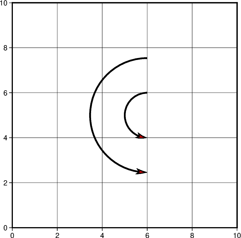
Much like when plotting Cartesian vectors, the default unit used is centimeters. When this is changed to inches, the size of the plot appears larger when the projection units do not change. Below is an example of two circular vectors. One is plotted using the default unit, and the second is plotted using inches. Despite using the same list to plot the vectors, a different measurement unit causes one to be larger than the other.
circular_vector = [6, 5, 1, 90, 270]

fig = pygmt.Figure()
fig.plot(
    region=[0, 10, 0, 10],
    projection="X10c",
    frame="ag",
    data=[circular_vector],
    style="m0.5c+ea",
    pen="2p",
    color="red3",
)

with pygmt.config(PROJ_LENGTH_UNIT="i"):
    fig.plot(
        data=[circular_vector],
        style="m0.5c+ea",
        pen="2p",
        color="red3",
    )
fig.show()
Out:
<IPython.core.display.Image object>
Plot Geographic Vectors
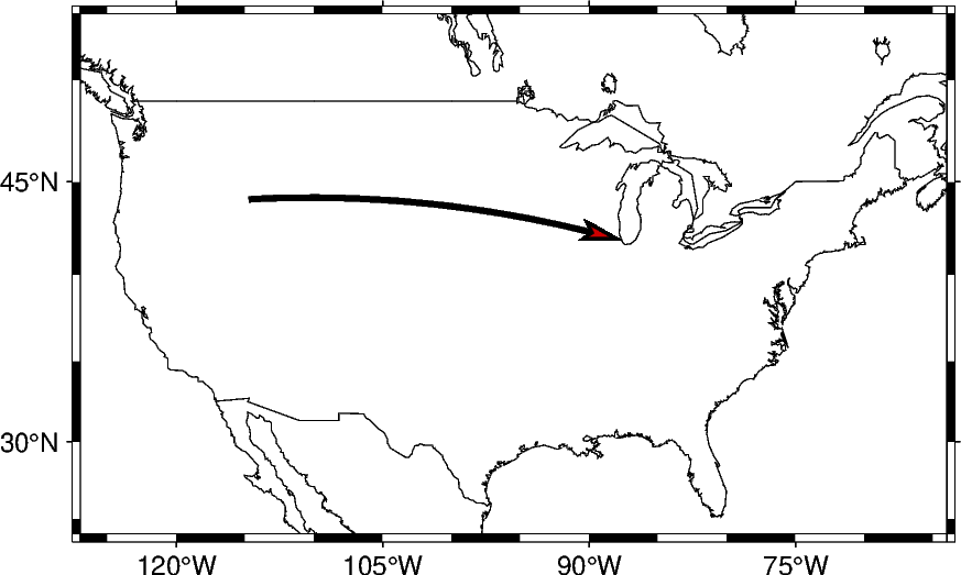
On this map,
point_1 and point_2 are coordinate pairs used to set the
start and end points of the geographic vector.
The geographical vector is going from Idaho to
Chicago. To style geographic
vectors, use = at the beginning of the style parameter.
Other styling features such as vector stem thickness and head color
can be passed into the pen and color parameters.
Note that the +s is added to use a startpoint and an endpoint to represent the vector instead of input angle and length.
point_1 = [-114.7420, 44.0682]
point_2 = [-87.6298, 41.8781]
data = np.array([point_1 + point_2])

fig = pygmt.Figure()
fig.coast(
    region=[-127, -64, 24, 53],
    projection="M10c",
    frame=True,
    borders=1,
    shorelines="0.25p,black",
    area_thresh=4000,
)
fig.plot(
    data=data,
    style="=0.5c+ea+s",
    pen="2p",
    color="red3",
)
fig.show()
Out:
<IPython.core.display.Image object>
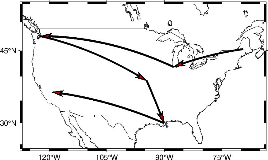
Using the same technique shown in the previous example,
multiple vectors can be plotted in a chain where the endpoint
of one is the starting point of another. This can be done
by adding the coordinate lists together to create this structure:
[[start_latitude, start_longitude, end_latitude, end_longitude]].
Each list within the 2D list contains the start and end information
for each vector.
# Coordinate pairs for all the locations used
ME = [-69.4455, 45.2538]
CHI = [-87.6298, 41.8781]
SEA = [-122.3321, 47.6062]
NO = [-90.0715, 29.9511]
KC = [-94.5786, 39.0997]
CA = [-119.4179, 36.7783]

# Add array to piece together the vectors
data = [ME + CHI, CHI + SEA, SEA + KC, KC + NO, NO + CA]

fig = pygmt.Figure()
fig.coast(
    region=[-127, -64, 24, 53],
    projection="M10c",
    frame=True,
    borders=1,
    shorelines="0.25p,black",
    area_thresh=4000,
)
fig.plot(
    data=data,
    style="=0.5c+ea+s",
    pen="2p",
    color="red3",
)
fig.show()
Out:
<IPython.core.display.Image object>
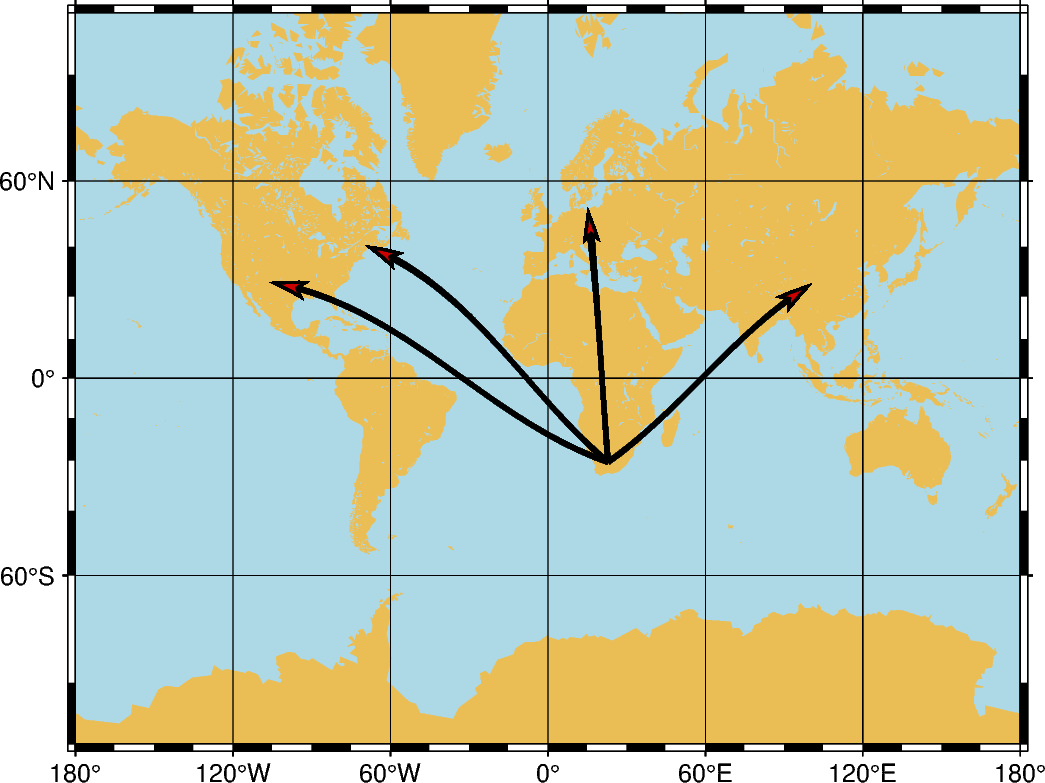
This example plots vectors over a Mercator projection. The starting points are located at SA which is South Africa and going to four different locations.
SA = [22.9375, -30.5595]
EUR = [15.2551, 54.5260]
ME = [-69.4455, 45.2538]
AS = [100.6197, 34.0479]
NM = [-105.8701, 34.5199]
data = np.array([SA + EUR, SA + ME, SA + AS, SA + NM])

fig = pygmt.Figure()
fig.coast(
    region=[-180, 180, -80, 80],
    projection="M0/0/12c",
    frame="afg",
    land="lightbrown",
    water="lightblue",
)
fig.plot(
    data=data,
    style="=0.5c+ea+s",
    pen="2p",
    color="red3",
)
fig.show()
Out:
<IPython.core.display.Image object>
Total running time of the script: ( 0 minutes 13.568 seconds)