Note
Go to the end to download the full example code.
Making subplots
When you’re preparing a figure for a paper, there will often be times when you’ll need to put many individual plots into one large figure, and tag them ‘abcd’. These individual plots are called subplots.
There are two main ways to create subplots in GMT:
Use
pygmt.Figure.shift_originto manually move each individual plot to the right position.Use
pygmt.Figure.subplotto define the layout of the subplots.
The first method is easier to use and should handle simple cases involving a couple of
subplots. For more advanced subplot layouts, however, we recommend the use of
pygmt.Figure.subplot which offers finer grained control, and this is what the
tutorial below will cover.
Let’s start by initializing a pygmt.Figure instance.
fig = pygmt.Figure()
Define subplot layout
The pygmt.Figure.subplot method is used to set up the layout, size, and other
attributes of the figure. It divides the whole canvas into regular grid areas with
n rows and m columns. Each grid area can contain an individual subplot. For
example:
 with fig.subplot(
     nrows=2,
     ncols=3,
     figsize=("15c", "6c"),
     frame=Frame(axes="lrtb"),
):
     ...
will define our figure to have a 2 row and 3 column grid layout.
figsize=("15c", "6c") defines the overall size of the figure to be 15 cm wide by
6 cm high. Using frame=Frame(axes="lrtb") allows us to customize the map frame for
all subplots instead of setting them individually. The figure layout will look like
the following:
with fig.subplot(nrows=2, ncols=3, figsize=("15c", "6c"), frame=Frame(axes="lrtb")):
    for i in range(2):  # row number starting from 0
        for j in range(3):  # column number starting from 0
            index = i * 3 + j  # index number starting from 0
            with fig.set_panel(panel=index):  # sets the current panel
                fig.text(
                    position="MC",
                    text=f"index: {index}; row: {i}, col: {j}",
                    region=[0, 1, 0, 1],
                )
fig.show()
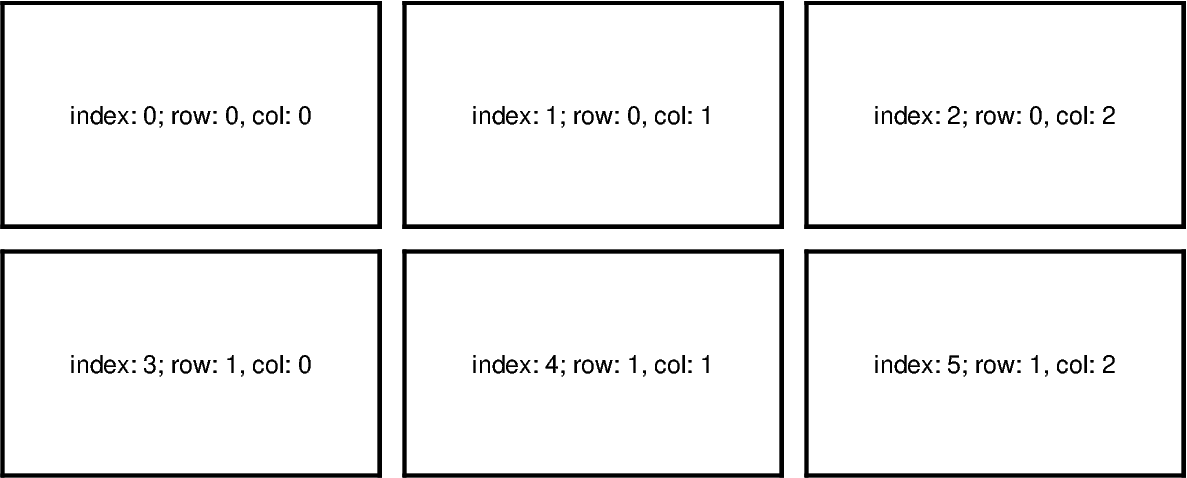
The pygmt.Figure.set_panel method activates a specified subplot, and all
subsequent plotting methods will take place in that subplot panel. This is similar to
matplotlib’s plt.sca method. In order to specify a subplot, you will need to
provide the identifier for that subplot via the panel parameter. Pass in either
the index number, or a tuple/list like (row, col) to panel.
Note
The row and column numbering starts from 0. So for a subplot layout with N rows and M columns, row numbers will go from 0 to N-1, and column numbers will go from 0 to M-1.
For example, to activate the subplot on the top right corner (index: 2) at row=0 and col=2, so that all subsequent plotting commands happen there, you can use the following command:
with fig.set_panel(panel=(0, 2)):
    ...
Making your first subplot
Next, let’s use what we learned above to make a 2 row by 2 column subplot figure. We’ll also pick up on some new parameters to configure our subplot.
fig = pygmt.Figure()
with fig.subplot(
    nrows=2,
    ncols=2,
    figsize=("15c", "6c"),
    tag=True,
    frame=Frame(axes="WSne", axis=Axis(annot=True, tick=True)),
    margins=["0.1c", "0.2c"],
    title="My Subplot Heading",
):
    fig.basemap(region=[0, 10, 0, 10], projection="X?", panel=[0, 0])
    fig.basemap(region=[0, 20, 0, 10], projection="X?", panel=[0, 1])
    fig.basemap(region=[0, 10, 0, 20], projection="X?", panel=[1, 0])
    fig.basemap(region=[0, 20, 0, 20], projection="X?", panel=[1, 1])
fig.show()
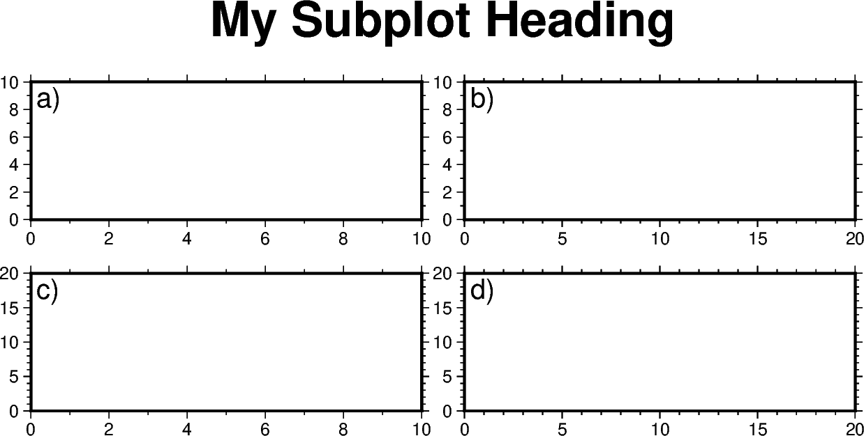
In this example, we define a 2-row, 2-column (2x2) subplot layout using
pygmt.Figure.subplot. The overall figure dimensions is set to be 15 cm wide
and 6 cm high (figsize=("15c", "6c")). In addition, we use some optional
parameters to fine-tune some details of the figure creation:
tag=True: Each subplot is automatically tagged ‘abcd’.margins=["0.1c", "0.2c"]: Adjusts the space between adjacent subplots. In this case, it is set as 0.1 cm in the x-direction and 0.2 cm in the y-direction.title="My Subplot Heading": Adds a title on top of the whole figure.
Notice that each subplot was set to use a linear projection "X?". Usually, we need
to specify the width and height of the map frame, but it is also possible to use a
question mark "?" to let GMT decide automatically on what is the most appropriate
width/height for each subplot’s map frame.
Tip
In the above example, we used the following commands to activate the four subplots explicitly one after another:
fig.basemap(..., panel=[0, 0])
fig.basemap(..., panel=[0, 1])
fig.basemap(..., panel=[1, 0])
fig.basemap(..., panel=[1, 1])
In fact, we can just use fig.basemap(..., panel=True) without specifying any
subplot index number, and GMT will automatically activate the next subplot panel.
Note
All plotting methods (e.g. pygmt.Figure.coast, pygmt.Figure.text,
etc) are able to use panel parameter when in subplot mode. Once a panel is
activated using panel or pygmt.Figure.set_panel, subsequent plotting
commands that don’t set a panel will have their elements added to the same
panel as before.
Shared x- and y-axes
In the example above with the four subplots, the two subplots for each row have the
same y-axis range, and the two subplots for each column have the same x-axis range.
You can use the sharex/sharey parameters to set a common x- and/or y-axis
between subplots.
fig = pygmt.Figure()
with fig.subplot(
    nrows=2,
    ncols=2,
    figsize=("15c", "6c"),  # width of 15 cm, height of 6 cm
    tag=True,
    margins=["0.3c", "0.2c"],  # horizontal 0.3 cm and vertical 0.2 cm margins
    title="My Subplot Heading",
    sharex="b",  # shared x-axis on the bottom side
    sharey="l",  # shared y-axis on the left side
    frame=Frame(axes="WSrt"),
):
    fig.basemap(region=[0, 10, 0, 10], projection="X?", panel=True)
    fig.basemap(region=[0, 20, 0, 10], projection="X?", panel=True)
    fig.basemap(region=[0, 10, 0, 20], projection="X?", panel=True)
    fig.basemap(region=[0, 20, 0, 20], projection="X?", panel=True)
fig.show()
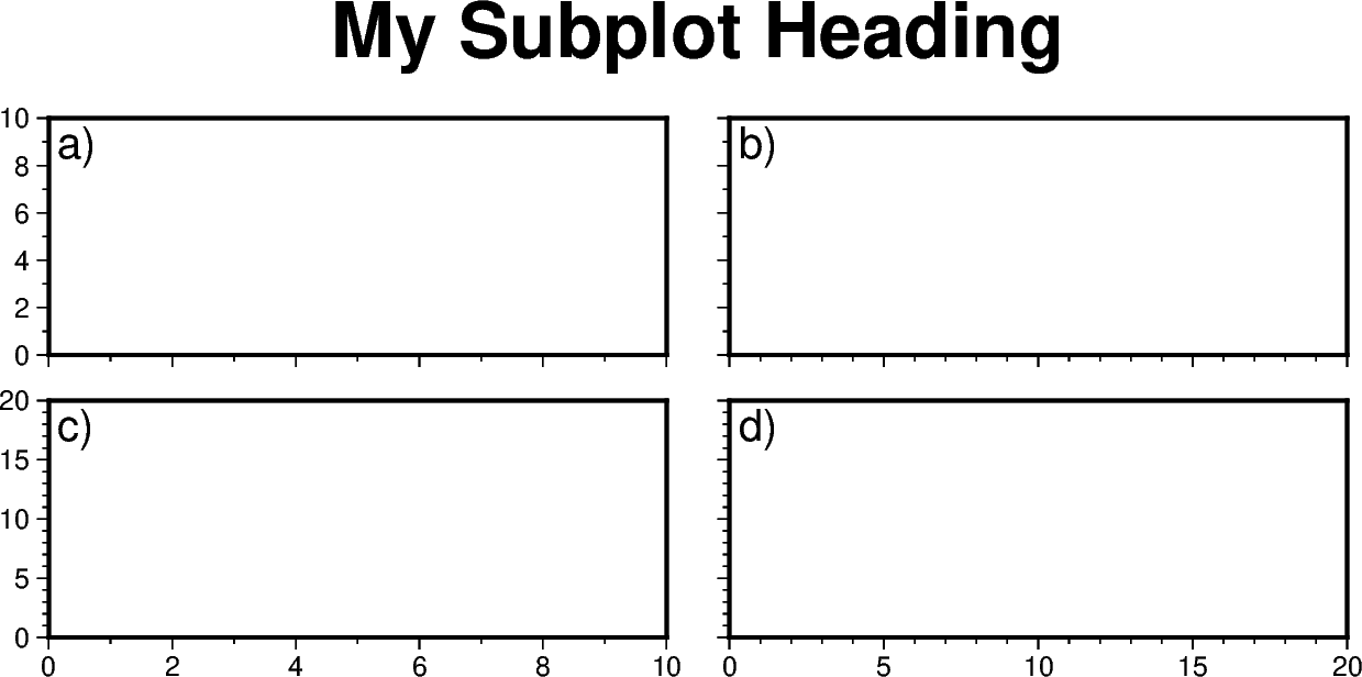
sharex="b" indicates that subplots in a column will share the x-axis, and only the
bottom axis is displayed. sharey="l" indicates that subplots within a row
will share the y-axis, and only the left axis is displayed.
Of course, instead of using the sharex/sharey parameters, you can also set a
different frame for each subplot to control the axis properties individually for
each subplot.
Advanced subplot layouts
Nested subplots are currently not supported. If you want to create more complex subplot layouts, some manual adjustments are needed.
The following example draws three subplots in a 2-row, 2-column layout, with the first subplot occupying the first row.
fig = pygmt.Figure()
# Bottom row, two subplots
with fig.subplot(nrows=1, ncols=2, figsize=("15c", "3c"), tag="b)"):
    fig.basemap(
        region=[0, 5, 0, 5],
        projection="X?",
        frame=Frame(axes="WSne", axis=Axis(annot=True, tick=True)),
        panel=[0, 0],
    )
    fig.basemap(
        region=[0, 5, 0, 5],
        projection="X?",
        frame=Frame(axes="WSne", axis=Axis(annot=True, tick=True)),
        panel=[0, 1],
    )
# Move plot origin by 1 cm above the height of the entire figure
fig.shift_origin(yshift="h+1c")
# Top row, one subplot
with fig.subplot(nrows=1, ncols=1, figsize=("15c", "3c"), tag="a)"):
    fig.basemap(
        region=[0, 10, 0, 10],
        projection="X?",
        frame=Frame(axes="WSne", axis=Axis(annot=True, tick=True)),
        panel=[0, 0],
    )
    fig.text(text="TEXT", x=5, y=5)

fig.show()
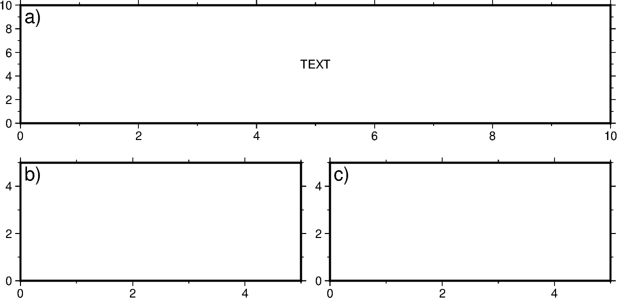
We start by drawing the bottom two subplots, setting tag="b)" so that the subplots
are tagged ‘b)’ and ‘c)’. Next, we use pygmt.Figure.shift_origin to move the
plot origin 1 cm above the height of the entire figure that is currently plotted
(i.e. the bottom row subplots). A single subplot is then plotted on the top row. You
may need to adjust the yshift parameter to make your plot look nice. This top row
uses tag="a)", and we also plotted some text inside. Note that projection="X?"
was used to let GMT automatically determine the size of the subplot according to the
size of the subplot area.
You can also manually override the tag for each subplot using for example,
fig.set_panel(..., tag="b) Panel 2") which would allow you to manually tag a
single subplot as you wish. This can be useful for adding a more descriptive subtitle
to individual subplots.
Total running time of the script: (0 minutes 0.598 seconds)