Note
Go to the end to download the full example code.
Interactive data visualization using Panel
Note
Please run the following code examples in a notebook environment otherwise the interactive parts of this tutorial will not work. You can use the button “Download Jupyter notebook” at the bottom of this page to download this script as a Jupyter notebook.
The library Panel can be used to
create interactive dashboards by connecting user-defined widgets to plots.
Panel can be used as an extension to Jupyter notebook/lab.
This tutorial is split into three parts:
Make a static map
Make an interactive map
Add a grid for Earth relief
Import the required packages
import numpy as np
import panel as pn
import pygmt

pn.extension()
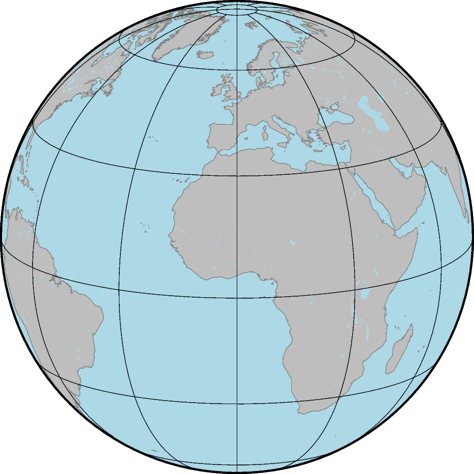
Make a static map
The Orthographic projection
can be used to show the Earth as a globe. Land and water masses are
filled with colors via the land and water parameters of
pygmt.Figure.coast, respectively. Coastlines are added using the
shorelines parameter.
# Create a new instance or object of the pygmt.Figure() class
fig = pygmt.Figure()
fig.coast(
    # Orthographic projection (G) with projection center at 0° East and
    # 15° North and a width of 12 centimeters
    projection="G0/15/12c",
    region="g",  # global
    frame="g30",  # Add frame and gridlines in steps of 30 degrees on top
    land="gray",  # Color land masses in "gray"
    water="lightblue",  # Color water masses in "lightblue"
    # Add coastlines with a 0.25-point thick pen in "gray50"
    shorelines="1/0.25p,gray50",
)
fig.show()
Make an interactive map
To generate a rotation of the Earth around the vertical axis, the central
longitude of the Orthographic projection is varied iteratively in steps of
10 degrees. The library Panel is used to create an interactive dashboard
with a slider (works only in a notebook environment, e.g., Jupyter notebook).
# Create a slider
slider_lon = pn.widgets.DiscreteSlider(
    name="Central longitude",  # Give name for quantity shown at the slider
    options=list(np.arange(0, 361, 10)),  # Range corresponding to longitude
    value=0,  # Set start value
)


@pn.depends(central_lon=slider_lon)
def view(central_lon):
    """
    Define a function for plotting the single slices.
    """
    # Create a new instance or object of the pygmt.Figure() class
    fig = pygmt.Figure()
    fig.coast(
        # Vary the central longitude used for the Orthographic projection
        projection=f"G{central_lon}/15/12c",
        region="g",
        frame="g30",
        land="gray",
        water="lightblue",
        shorelines="1/0.25p,gray50",
    )
    return fig


# Make an interactive dashboard
pn.Column(slider_lon, view)
Column
    [0] DiscreteSlider(formatter='%d', name='Central longitude', options=[np.int64(0), ...], value=0)
    [1] ParamFunction(function, _pane=PNG, defer_load=False)
Add a grid for Earth relief
Instead of using colors as fill for the land and water masses a grid can be displayed. Here, the Earth relief is shown by color-coding the elevation.
# Download a grid for Earth relief with a resolution of 10 arc-minutes
grd_relief = pygmt.datasets.load_earth_relief(resolution="10m")

# Create a slider
slider_lon = pn.widgets.DiscreteSlider(
    name="Central longitude",
    options=list(np.arange(0, 361, 10)),
    value=0,
)


@pn.depends(central_lon=slider_lon)
def view(central_lon):
    """
    Define a function for plotting the single slices.
    """
    # Create a new instance or object of the pygmt.Figure() class
    fig = pygmt.Figure()
    # Set up a colormap for the elevation in meters
    pygmt.makecpt(
        cmap="SCM/oleron",
        # minimum, maximum, step
        series=[int(grd_relief.data.min()) - 1, int(grd_relief.data.max()) + 1, 100],
    )
    # Plot the grid for the elevation
    fig.grdimage(
        projection=f"G{central_lon}/15/12c",
        region="g",
        grid=grd_relief,  # Use grid downloaded above
        cmap=True,  # Use colormap defined above
        frame="g30",
    )
    # Add a horizontal colorbar for the elevation
    # with annotations (a) in steps of 2000 and ticks (f) in steps of 1000
    # and labels (+l) at the x-axis "Elevation" and y-axis "m" (meters)
    fig.colorbar(frame=["a2000f1000", "x+lElevation", "y+lm"])
    return fig


# Make an interactive dashboard
pn.Column(slider_lon, view)
Column
    [0] DiscreteSlider(formatter='%d', name='Central longitude', options=[np.int64(0), ...], value=0)
    [1] ParamFunction(function, _pane=PNG, defer_load=False)
Total running time of the script: (0 minutes 1.794 seconds)