Note
Click here to download the full example code
Performing grid histogram equalization
The pygmt.grdhisteq.equalize_grid function creates a grid using
statistics based on a cumulative distribution function.
import pygmt
Load sample data
Load the sample Earth relief data for a region around Yosemite valley
and use pygmt.grd2xyz to create a pandas.Series with the
z values.
grid = pygmt.datasets.load_earth_relief(
    resolution="03s", region=[-119.825, -119.4, 37.6, 37.825]
)
grid_dist = pygmt.grd2xyz(grid=grid, output_type="pandas")["elevation"]
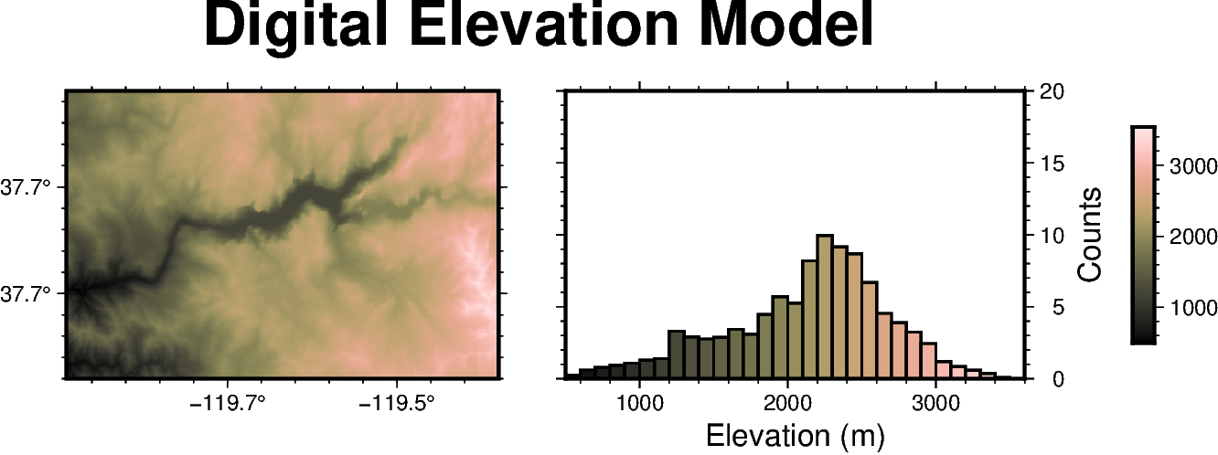
Plot the original digital elevation model and data distribution
For comparison, we will create a map of the original digital elevation model and a histogram showing the distribution of elevation data values.
# Create an instance of the Figure class
fig = pygmt.Figure()
# Define figure configuration
pygmt.config(FORMAT_GEO_MAP="ddd.x", MAP_FRAME_TYPE="plain")
# Define the colormap for the figure
pygmt.makecpt(series=[500, 3540], cmap="turku")
# Setup subplots with two panels
with fig.subplot(
    nrows=1, ncols=2, figsize=("13.5c", "4c"), title="Digital Elevation Model"
):
    # Plot the original digital elevation model in the first panel
    with fig.set_panel(panel=0):
        fig.grdimage(grid=grid, projection="M?", frame="WSne", cmap=True)
    # Plot a histogram showing the z-value distribution in the original digital
    # elevation model
    with fig.set_panel(panel=1):
        fig.histogram(
            data=grid_dist,
            projection="X?",
            region=[500, 3600, 0, 20],
            series=[500, 3600, 100],
            frame=["wnSE", "xaf+lElevation (m)", "yaf+lCounts"],
            cmap=True,
            histtype=1,
            pen="1p,black",
        )
        fig.colorbar(position="JMR+o1.5c/0c+w3c/0.3c", frame=True)
fig.show()
Out:
<IPython.core.display.Image object>
Equalize grid based on a linear distribution
The pygmt.grdhisteq.equalize_grid method creates a new grid with the
z-values representing the position of the original z-values in a given
cumulative distribution. By default, it computes the position in a linear
distribution. Here, we equalize the grid into nine divisions based on a
linear distribution and produce a pandas.Series with the z-values
for the new grid.
divisions = 9
linear = pygmt.grdhisteq.equalize_grid(grid=grid, divisions=divisions)
linear_dist = pygmt.grd2xyz(grid=linear, output_type="pandas")["z"]
Calculate the bins used for data transformation
The pygmt.grdhisteq.compute_bins method reports statistics about the
grid equalization. Here, we report the bins that would linearly divide the
original data into 9 divisions with equal area. In our new grid produced by
pygmt.grdhisteq.equalize_grid, all the grid cells with values between
start and stop of bin_id=0 are assigned the value 0, all grid
cells with values between start and stop of bin_id=1 are assigned
the value 1, and so on.
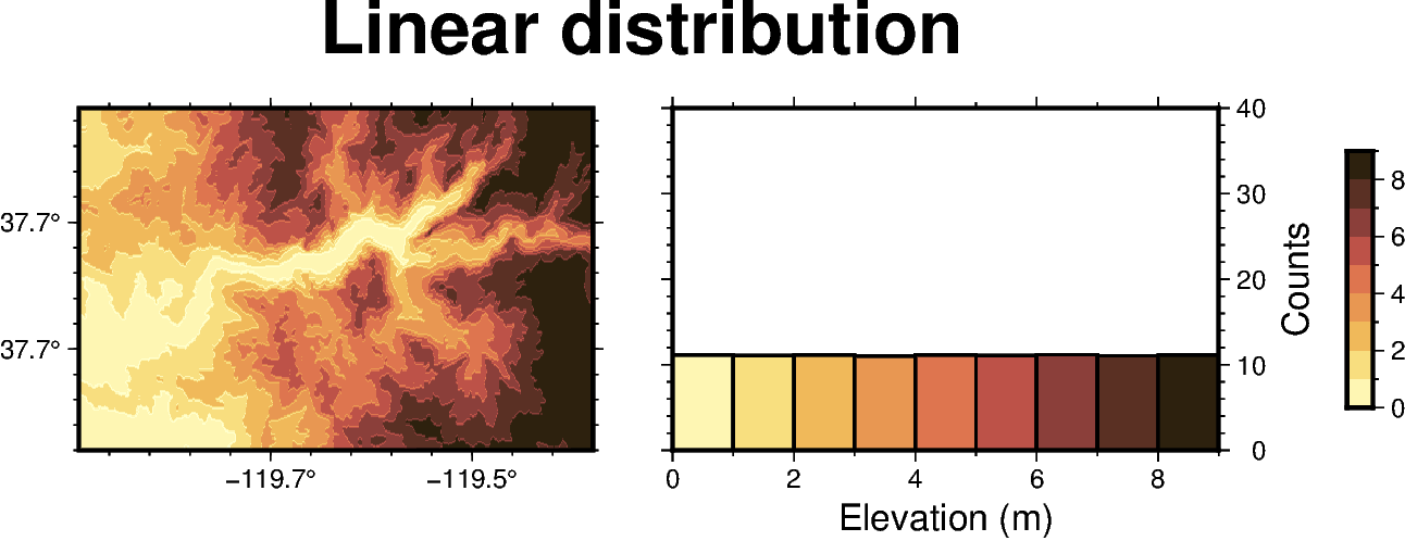
Plot the equally distributed data
Here we create a map showing the grid that has been transformed to have a linear distribution with nine divisions and a histogram of the data values.
# Create an instance of the Figure class
fig = pygmt.Figure()
# Define figure configuration
pygmt.config(FORMAT_GEO_MAP="ddd.x", MAP_FRAME_TYPE="plain")
# Define the colormap for the figure
pygmt.makecpt(series=[0, divisions, 1], cmap="lajolla")
# Setup subplots with two panels
with fig.subplot(
    nrows=1, ncols=2, figsize=("13.5c", "4c"), title="Linear distribution"
):
    # Plot the grid with a linear distribution in the first panel
    with fig.set_panel(panel=0):
        fig.grdimage(grid=linear, projection="M?", frame="WSne", cmap=True)
    # Plot a histogram showing the linear z-value distribution
    with fig.set_panel(panel=1):
        fig.histogram(
            data=linear_dist,
            projection="X?",
            region=[0, divisions, 0, 40],
            series=[0, divisions, 1],
            frame=["wnSE", "xaf+lElevation (m)", "yaf+lCounts"],
            cmap=True,
            histtype=1,
            pen="1p,black",
        )
        fig.colorbar(position="JMR+o1.5c/0c+w3c/0.3c", frame=True)
fig.show()
Out:
<IPython.core.display.Image object>
Transform grid based on a normal distribution
The gaussian parameter of pygmt.grdhisteq.equalize_grid can be
used to transform the z-values relative to their position in a normal
distribution rather than a linear distribution. In this case, the output
data are continuous rather than discrete.
normal = pygmt.grdhisteq.equalize_grid(grid=grid, gaussian=True)
normal_dist = pygmt.grd2xyz(grid=normal, output_type="pandas")["z"]
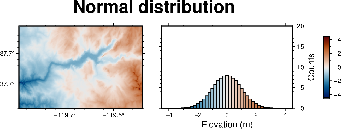
Plot the normally distributed data
Here we create a map showing the grid that has been transformed to have a normal distribution and a histogram of the data values.
# Create an instance of the Figure class
fig = pygmt.Figure()
# Define figure configuration
pygmt.config(FORMAT_GEO_MAP="ddd.x", MAP_FRAME_TYPE="plain")
# Define the colormap for the figure
pygmt.makecpt(series=[-4.5, 4.5], cmap="vik")
# Setup subplots with two panels
with fig.subplot(
    nrows=1, ncols=2, figsize=("13.5c", "4c"), title="Normal distribution"
):
    # Plot the grid with a normal distribution in the first panel
    with fig.set_panel(panel=0):
        fig.grdimage(grid=normal, projection="M?", frame="WSne", cmap=True)
    # Plot a histogram showing the normal z-value distribution
    with fig.set_panel(panel=1):
        fig.histogram(
            data=normal_dist,
            projection="X?",
            region=[-4.5, 4.5, 0, 20],
            series=[-4.5, 4.5, 0.2],
            frame=["wnSE", "xaf+lElevation (m)", "yaf+lCounts"],
            cmap=True,
            histtype=1,
            pen="1p,black",
        )
        fig.colorbar(position="JMR+o1.5c/0c+w3c/0.3c", frame=True)
fig.show()
Out:
<IPython.core.display.Image object>
Equalize grid based on a quadratic distribution
The quadratic parameter of pygmt.grdhisteq.equalize_grid can be
used to transform the z-values relative to their position in a quadratic
distribution rather than a linear distribution. Here, we equalize the grid
into nine divisions based on a quadratic distribution and produce a
pandas.Series with the z-values for the new grid.
quadratic = pygmt.grdhisteq.equalize_grid(
    grid=grid, quadratic=True, divisions=divisions
)
quadratic_dist = pygmt.grd2xyz(grid=quadratic, output_type="pandas")["z"]
Calculate the bins used for data transformation
We can also use the quadratic parameter of
pygmt.grdhisteq.compute_bins to report the bins used for dividing
the grid into 9 divisions based on their position in a quadratic
distribution.
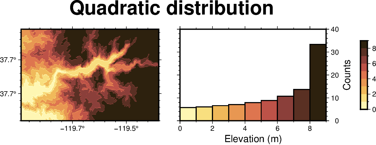
Plot the quadratic distribution of data
Here we create a map showing the grid that has been transformed to have a quadratic distribution and a histogram of the data values.
# Create an instance of the Figure class
fig = pygmt.Figure()
# Define figure configuration
pygmt.config(FORMAT_GEO_MAP="ddd.x", MAP_FRAME_TYPE="plain")
# Define the colormap for the figure
pygmt.makecpt(series=[0, divisions, 1], cmap="lajolla")
# Setup subplots with two panels
with fig.subplot(
    nrows=1, ncols=2, figsize=("13.5c", "4c"), title="Quadratic distribution"
):
    # Plot the grid with a quadratic distribution in the first panel
    with fig.set_panel(panel=0):
        fig.grdimage(grid=quadratic, projection="M?", frame="WSne", cmap=True)
    # Plot a histogram showing the quadratic z-value distribution
    with fig.set_panel(panel=1):
        fig.histogram(
            data=quadratic_dist,
            projection="X?",
            region=[0, divisions, 0, 40],
            series=[0, divisions, 1],
            frame=["wnSE", "xaf+lElevation (m)", "yaf+lCounts"],
            cmap=True,
            histtype=1,
            pen="1p,black",
        )
        fig.colorbar(position="JMR+o1.5c/0c+w3c/0.3c", frame=True)
fig.show()
Out:
<IPython.core.display.Image object>
Total running time of the script: ( 0 minutes 11.675 seconds)