Note
Click here to download the full example code
Plotting Earth relief
Plotting a map of Earth relief can use the data accessed by the
pygmt.datasets.load_earth_relief method. The data can then be plotted using the
pygmt.Figure.grdimage method.
Note
This tutorial assumes the use of a Python notebook, such as IPython or Jupyter Notebook.
To see the figures while using a Python script instead, use
fig.show(method="external) to display the figure in the default PDF viewer.
To save the figure, use fig.savefig("figname.pdf") where "figname.pdf"
is the desired name and file extension for the saved figure.
import pygmt
Load sample Earth relief data for the entire globe at a resolution of 1 arc degree. The other available resolutions are show at https://docs.generic-mapping-tools.org/latest/datasets/remote-data.html#global-earth-relief-grids.
grid = pygmt.datasets.load_earth_relief(resolution="01d")
Create a plot
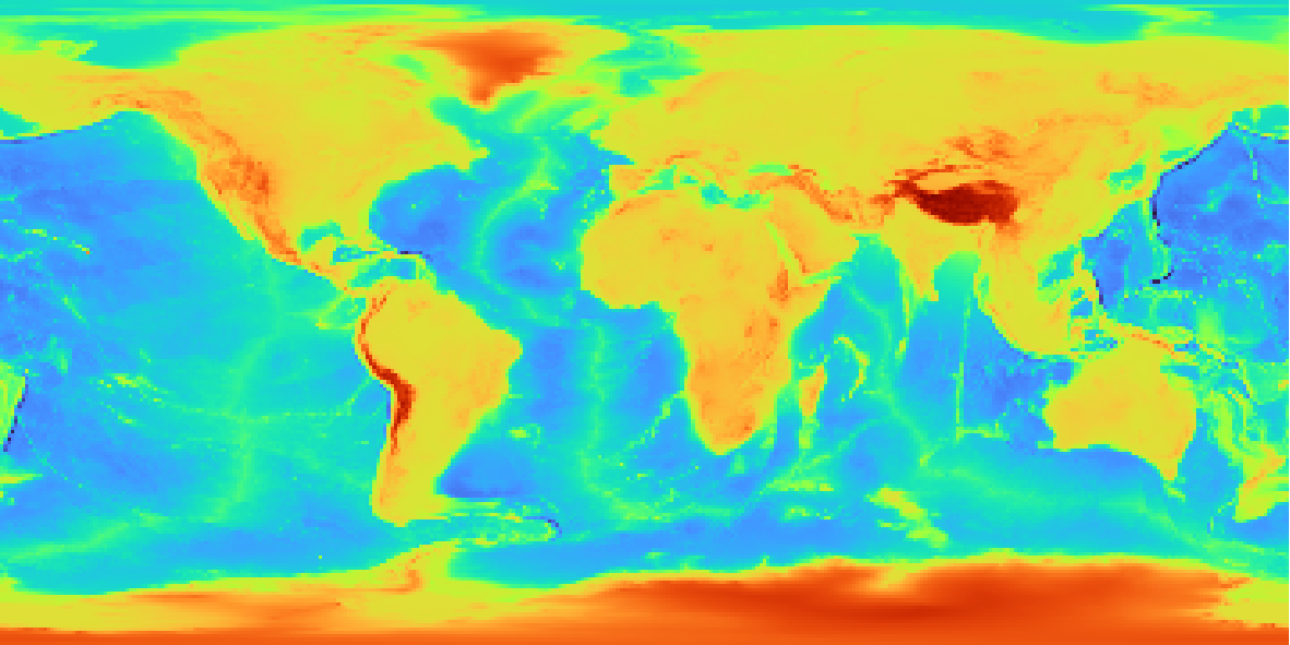
The pygmt.Figure.grdimage method takes the grid input to
create a figure. It creates and applies a color palette to the figure based upon the
z-values of the data. By default, it plots the map with the turbo CPT, an
equidistant cylindrical projection, and with no frame.
fig = pygmt.Figure()
fig.grdimage(grid=grid)
fig.show()
Out:
<IPython.core.display.Image object>
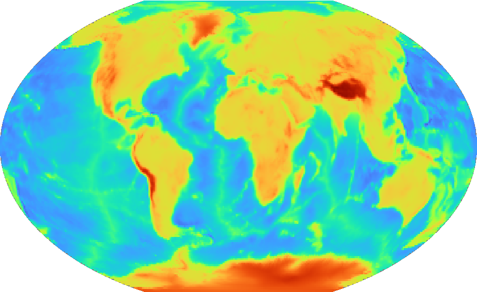
pygmt.Figure.grdimage can take the optional argument projection for the
map. In the example below, the projection is set as R12c for 12 centimeter
figure with a Winkel Tripel projection. For a list of available projections,
see https://docs.generic-mapping-tools.org/latest/cookbook/map-projections.html.
fig = pygmt.Figure()
fig.grdimage(grid=grid, projection="R12c")
fig.show()
Out:
<IPython.core.display.Image object>
Set a color map
pygmt.Figure.grdimage takes the cmap argument to set the CPT of the
figure. Examples of common CPTs for Earth relief are shown below.
A full list of CPTs can be found at https://docs.generic-mapping-tools.org/latest/cookbook/cpts.html.
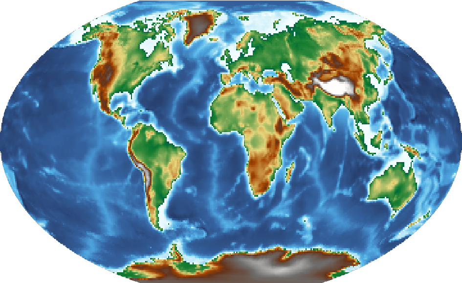
Using the geo CPT:
fig = pygmt.Figure()
fig.grdimage(grid=grid, projection="R12c", cmap="geo")
fig.show()
Out:
<IPython.core.display.Image object>
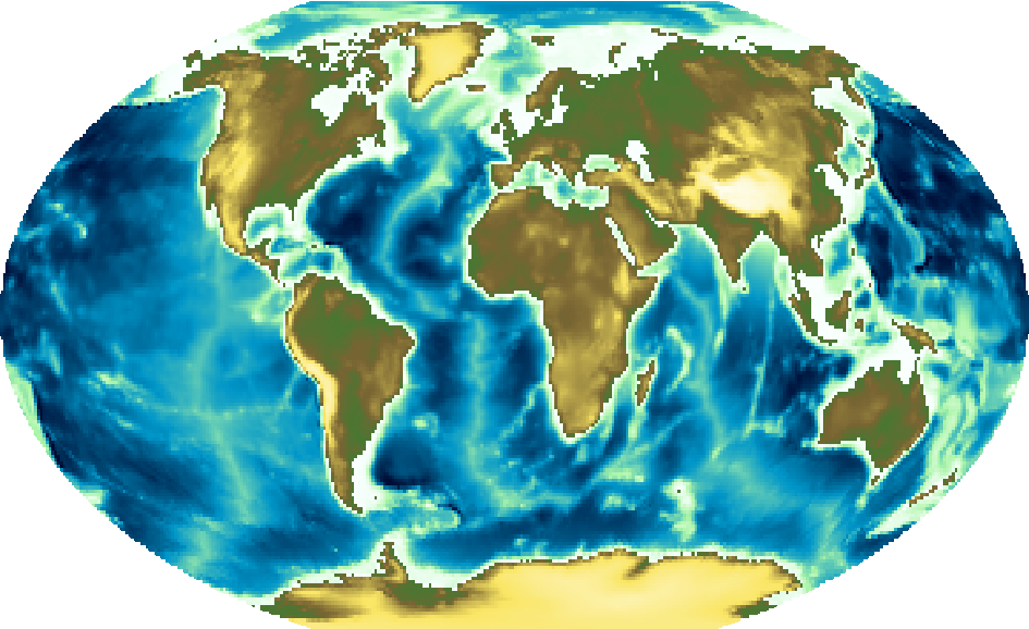
Using the relief CPT:
fig = pygmt.Figure()
fig.grdimage(grid=grid, projection="R12c", cmap="relief")
fig.show()
Out:
<IPython.core.display.Image object>
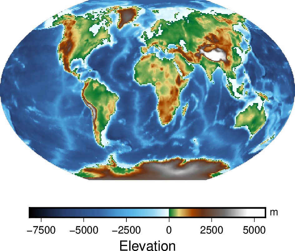
Add a color bar
The pygmt.Figure.colorbar method displays the CPT and the associated Z-values
of the figure, and by default uses the same CPT set by the cmap argument
for pygmt.Figure.grdimage. The frame argument for
pygmt.Figure.colorbar can be used to set the axis intervals and labels. A
list is used to pass multiple arguments to frame. In the example below,
a2500 sets the axis interval to 2,500, x+lElevation sets the x-axis
label, and y+lm sets the y-axis label.
fig = pygmt.Figure()
fig.grdimage(grid=grid, projection="R12c", cmap="geo")
fig.colorbar(frame=["a2500", "x+lElevation", "y+lm"])
fig.show()
Out:
<IPython.core.display.Image object>
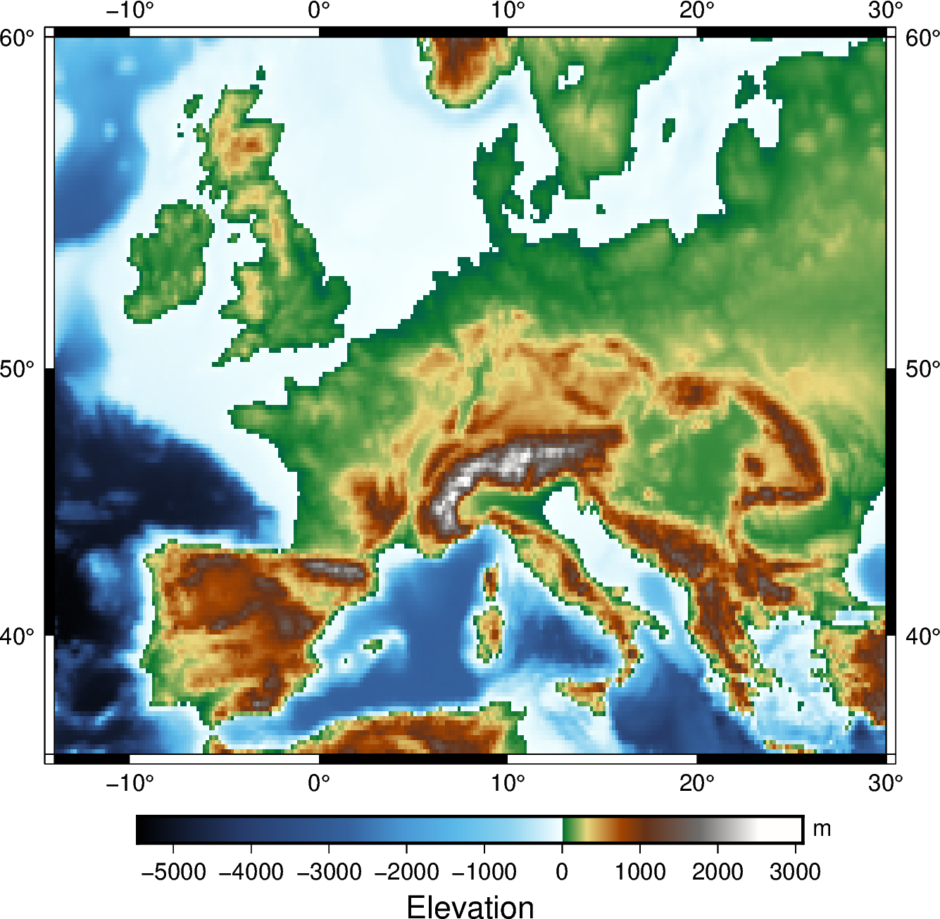
Create a region map
In addition to providing global data, the region argument for
pygmt.datasets.load_earth_relief can be used to provide data for a specific
area. The region argument is required for resolutions at 5 arc minutes or higher,
and accepts a list (as in the example below) or a string. The geographic ranges are
passed as xmin/xmax/ymin/ymax.
The example below uses data with a 10 arc minute resolution, and plots it on a
15 centimeter figure with a Mercator projection and a CPT set to geo.
frame="a" is used to add a frame to the figure.
grid = pygmt.datasets.load_earth_relief(resolution="10m", region=[-14, 30, 35, 60])
fig = pygmt.Figure()
fig.grdimage(grid=grid, projection="M15c", frame="a", cmap="geo")
fig.colorbar(frame=["a1000", "x+lElevation", "y+lm"])
fig.show()
Out:
<IPython.core.display.Image object>
Total running time of the script: ( 0 minutes 7.525 seconds)