Note
Click here to download the full example code
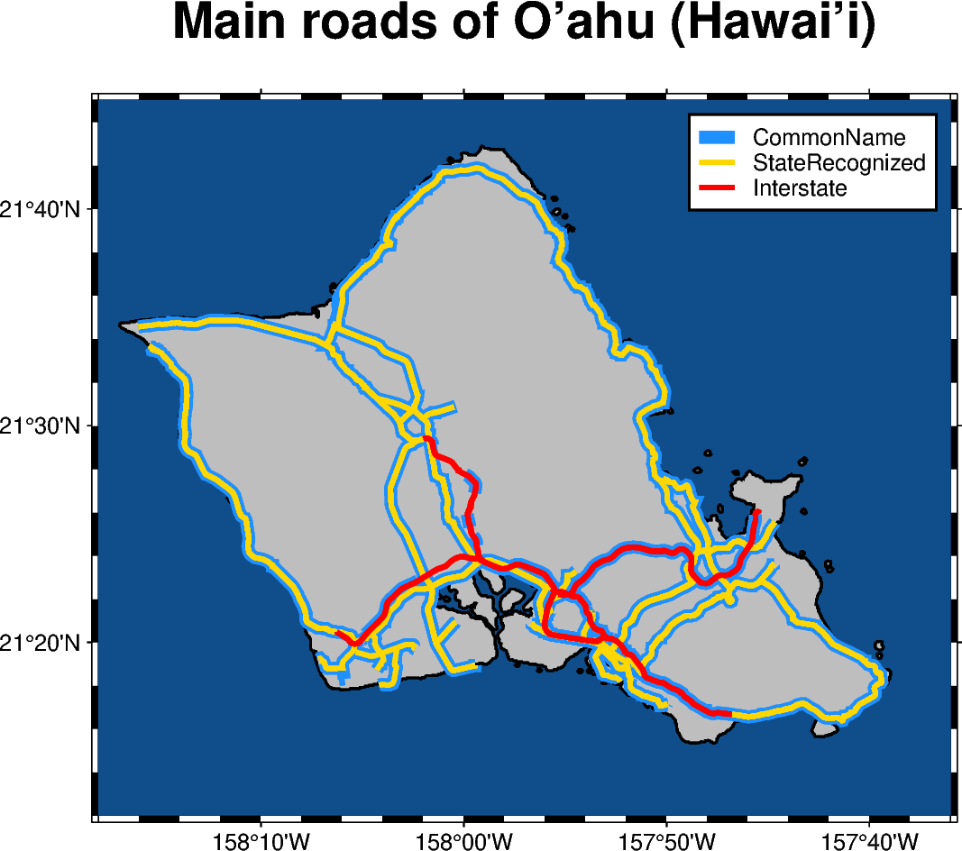
Roads
The pygmt.Figure.plot method allows us to plot geographical data such
as lines which are stored in a geopandas.GeoDataFrame object. Use
geopandas.read_file to load data from any supported OGR format such as
a shapefile (.shp), GeoJSON (.geojson), geopackage (.gpkg), etc. Then, pass the
geopandas.GeoDataFrame as an argument to the data parameter in
pygmt.Figure.plot, and style the geometry using the pen parameter.
Out:
/usr/share/miniconda3/envs/pygmt/lib/python3.9/site-packages/geopandas/io/file.py:362: FutureWarning: pandas.Int64Index is deprecated and will be removed from pandas in a future version. Use pandas.Index with the appropriate dtype instead.
  pd.Int64Index,
/usr/share/miniconda3/envs/pygmt/lib/python3.9/site-packages/geopandas/io/file.py:362: FutureWarning: pandas.Int64Index is deprecated and will be removed from pandas in a future version. Use pandas.Index with the appropriate dtype instead.
  pd.Int64Index,
/usr/share/miniconda3/envs/pygmt/lib/python3.9/site-packages/geopandas/io/file.py:362: FutureWarning: pandas.Int64Index is deprecated and will be removed from pandas in a future version. Use pandas.Index with the appropriate dtype instead.
  pd.Int64Index,
<IPython.core.display.Image object>
import geopandas as gpd
import pygmt

# Read shapefile data using geopandas
gdf = gpd.read_file(
    "http://www2.census.gov/geo/tiger/TIGER2015/PRISECROADS/tl_2015_15_prisecroads.zip"
)
# The dataset contains different road types listed in the RTTYP column,
# here we select the following ones to plot:
roads_common = gdf[gdf.RTTYP == "M"]  # Common name roads
roads_state = gdf[gdf.RTTYP == "S"]  # State recognized roads
roads_interstate = gdf[gdf.RTTYP == "I"]  # Interstate roads

fig = pygmt.Figure()

# Define target region around O'ahu (Hawai'i)
region = [-158.3, -157.6, 21.2, 21.75]  # xmin, xmax, ymin, ymax

title = r"Main roads of O\047ahu (Hawai\047i)"  # \047 is octal code for '
fig.basemap(region=region, projection="M12c", frame=["af", f'WSne+t"{title}"'])
fig.coast(land="gray", water="dodgerblue4", shorelines="1p,black")

# Plot the individual road types with different pen settings and assign labels
# which are displayed in the legend
fig.plot(data=roads_common, pen="5p,dodgerblue", label="CommonName")
fig.plot(data=roads_state, pen="2p,gold", label="StateRecognized")
fig.plot(data=roads_interstate, pen="2p,red", label="Interstate")

# Add legend
fig.legend()

fig.show()
Total running time of the script: ( 0 minutes 3.710 seconds)