pygmt.Figure.grdimage
- Figure.grdimage(grid, monochrome=False, no_clip=False, projection=None, frame=False, region=None, verbose=False, panel=False, transparency=None, perspective=False, cores=False, **kwargs)
Project and plot grids or images.
Reads a 2-D grid file and produces a gray-shaded (or colored) map by building a rectangular image and assigning pixels a gray-shade (or color) based on the z-value and the CPT file. Optionally, illumination may be added by providing a file with intensities in the (-1,+1) range or instructions to derive intensities from the input data grid. Values outside this range will be clipped. Such intensity files can be created from the grid using
pygmt.grdgradientand, optionally, modified by https://docs.generic-mapping-tools.org/6.6/grdmath.html orpygmt.grdhisteq. Alternatively, pass image which can be an image file (geo-referenced or not). In this case the image can optionally be illuminated with the file provided via theshadingparameter. Here, if image has no coordinates then those of the intensity file will be used.When using map projections, the grid is first resampled on a new rectangular grid with the same dimensions. Higher resolution images can be obtained by using the
dpiparameter. To obtain the resampled value (and hence shade or color) of each map pixel, its location is inversely projected back onto the input grid after which a value is interpolated between the surrounding input grid values. By default bi-cubic interpolation is used. Aliasing is avoided by also forward projecting the input grid nodes. If two or more nodes are projected onto the same pixel, their average will dominate in the calculation of the pixel value. Interpolation and aliasing is controlled with theinterpolationparameter.The
regionparameter can be used to select a map region larger or smaller than that implied by the extent of the grid.Full GMT docs at https://docs.generic-mapping-tools.org/6.6/grdimage.html.
Aliases:
C = cmap
D = img_in
E = dpi
G = bitcolor
I = shading
Q = nan_transparent
f = coltypes
n = interpolation
B = frame
J = projection
M = monochrome
N = no_clip
R = region
V = verbose
c = panel
p = perspective
t = transparency
x = cores
- Parameters:
grid (
str|PathLike|DataArray) –Name of the input grid file or the grid loaded as a
xarray.DataArrayobject.For reading a specific grid file format or applying basic data operations, see https://docs.generic-mapping-tools.org/6.6/gmt.html#grd-inout-full for the available modifiers.
frame (bool, str, or list) – Set map boundary frame and axes attributes.
cmap (str) – File name of a CPT file or a series of comma-separated colors (e.g., color1,color2,color3) to build a linear continuous CPT from those colors automatically.
img_in (str) – [r]. GMT will automatically detect standard image files (Geotiff, TIFF, JPG, PNG, GIF, etc.) and will read those via GDAL. For very obscure image formats you may need to explicitly set
img_in, which specifies that the grid is in fact an image file to be read via GDAL. Append r to assign the region specified byregionto the image. For example, if you have usedregion="d"then the image will be assigned a global domain. This mode allows you to project a raw image (an image without referencing coordinates).dpi (int) – [i|dpi]. Set the resolution of the projected grid that will be created if a map projection other than Linear or Mercator was selected [Default is
100dpi]. By default, the projected grid will be of the same size (rows and columns) as the input file. Specify i to use the PostScript image operator to interpolate the image at the device resolution.bitcolor (str) – color[+b|f]. This parameter only applies when a resulting 1-bit image otherwise would consist of only two colors: black (0) and white (255). If so, this parameter will instead use the image as a transparent mask and paint the mask with the given color. Append +b to paint the background pixels (1) or +f for the foreground pixels [Default is +f].
shading (str or
xarray.DataArray) – [intensfile|intensity|modifiers]. Give the name of a grid file or a DataArray with intensities in the (-1,+1) range, or a constant intensity to apply everywhere (affects the ambient light). Alternatively, derive an intensity grid from the input data grid via a call topygmt.grdgradient; append +aazimuth, +nargs, and +mambient to specify azimuth, intensity, and ambient arguments for that function, or just give +d to select the default arguments (+a-45+nt1+m0). If you want a more specific intensity scenario then runpygmt.grdgradientseparately first. If we should derive intensities from another file than grid, specify the file with suitable modifiers [Default is no illumination]. Note: If the input data represent an image then an intensfile or constant intensity must be provided.projection (
str|None, default:None) – projcode[projparams/]width|scale. Select map projection.monochrome (
bool, default:False) – Force conversion to monochrome image using the (television) YIQ transformation. Cannot be used withnan_transparent.no_clip (
bool, default:False) – Do not clip the image at the frame boundaries (only relevant for non-rectangular maps) [Default isFalse].nan_transparent (bool or str) – [+zvalue][color] Make grid nodes with z = NaN transparent, using the color-masking feature in PostScript Level 3 (the PS device must support PS Level 3). If the input is a grid, use +z to select another grid value than NaN. If input is instead an image, append an alternate color to select another pixel value to be transparent [Default is
"black"].region (str or list) – xmin/xmax/ymin/ymax[+r][+uunit]. Specify the region of interest.
verbose (bool or str) – Select verbosity level [Full usage].
panel (
int|Sequence[int] |bool, default:False) –Select a specific subplot panel. Only allowed when used in
Figure.subplotmode.Trueto advance to the next panel in the selected order.index to specify the index of the desired panel.
(row, col) to specify the row and column of the desired panel.
The panel order is determined by the
Figure.subplotmethod. row, col and index all start at 0.coltypes (str) – [i|o]colinfo. Specify data types of input and/or output columns (time or geographical data). Full documentation is at https://docs.generic-mapping-tools.org/6.6/gmt.html#f-full.
interpolation (str) –
[b|c|l|n][+a][+bBC][+c][+tthreshold]. Select interpolation mode for grids. You can select the type of spline used:
b for B-spline
c for bicubic [Default]
l for bilinear
n for nearest-neighbor
perspective (
float|Sequence[float] |str|bool, default:False) –Select perspective view and set the azimuth and elevation of the viewpoint.
Accepts a single value or a sequence of two or three values: azimuth, (azimuth, elevation), or (azimuth, elevation, zlevel).
azimuth: Azimuth angle of the viewpoint in degrees [Default is 180, i.e., looking from south to north].
elevation: Elevation angle of the viewpoint above the horizon [Default is 90, i.e., looking straight down at nadir].
zlevel: Z-level at which 2-D elements (e.g., the map frame) are drawn. Only applied when used together with
zsizeorzscale. [Default is at the bottom of the z-axis].
Alternatively, set
perspective=Trueto reuse the perspective setting from the previous plotting method, or pass a string following the full GMT syntax for finer control (e.g., adding+wor+vmodifiers to select an axis location other than the plot origin). See https://docs.generic-mapping-tools.org/6.6/gmt.html#perspective-full for details.transparency (float) – Set transparency level, in [0-100] percent range [Default is
0, i.e., opaque]. Only visible when PDF or raster format output is selected. Only the PNG format selection adds a transparency layer in the image (for further processing).cores (
int|bool, default:False) – Specify the number of active cores to be used in any OpenMP-enabled multi-threaded algorithms. By default, all available cores are used. Set a positive number n to use n cores (if too large it will be truncated to the maximum cores available); or set a negative number -n to select (all - n) cores (or at least 1 if n equals or exceeds all).
Example
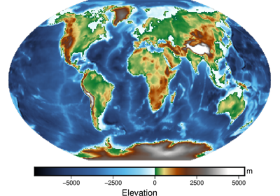
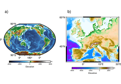
>>> import pygmt
>>> # load the 30 arc-minutes grid with "gridline" registration
>>> grid = pygmt.datasets.load_earth_relief("30m", registration="gridline")
>>> # create a new plot with pygmt.Figure()
>>> fig = pygmt.Figure()
>>> # pass in the grid and set the CPT to "geo"
>>> # set the projection to Mollweide and the size to 10 cm
>>> fig.grdimage(grid=grid, cmap="gmt/geo", projection="W10c", frame="ag")
>>> # show the plot
>>> fig.show()
Examples using pygmt.Figure.grdimage
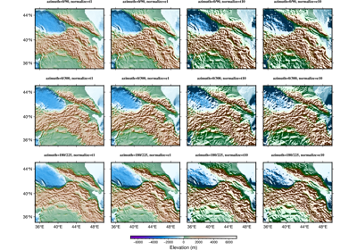
Calculating grid gradient with custom azimuth and normalize parameters