pygmt.Figure.grdview
- Figure.grdview(grid, cmap=None, drape_grid=None, surftype=None, dpi=None, nan_transparent=False, monochrome=False, contour_pen=None, mesh_fill=None, mesh_pen=None, plane=False, facade_fill=None, facade_pen=None, projection=None, smooth=None, zscale=None, zsize=None, region=None, frame=False, verbose=False, panel=False, perspective=False, transparency=None, **kwargs)
Create 3-D perspective image or surface mesh from a grid.
Reads a 2-D grid file and produces a 3-D perspective plot by drawing a mesh, painting a colored/gray-shaded surface made up of polygons, or by scanline conversion of these polygons to a raster image. Options include draping a data set on top of a surface, plotting of contours on top of the surface, and apply artificial illumination based on intensities provided in a separate grid file.
Full GMT docs at https://docs.generic-mapping-tools.org/6.6/grdview.html.
Aliases:
I = shading
f = coltypes
n = interpolation
B = frame
C = cmap
G = drape_grid
J = projection
Jz = zscale
JZ = zsize
N = plane, facade_fill
Q = surftype, dpi, mesh_fill, nan_transparent, +m: monochrome
R = region
S = smooth
V = verbose
Wc = contour_pen
Wf = facade_pen
Wm = mesh_pen
c = panel
p = perspective
t = transparency
- Parameters:
grid (
str|PathLike|DataArray) –Name of the input grid file or the grid loaded as a
xarray.DataArrayobject.For reading a specific grid file format or applying basic data operations, see https://docs.generic-mapping-tools.org/6.6/gmt.html#grd-inout-full for the available modifiers.
cmap (
str|None, default:None) – The name of the color palette table to use.drapegrid – The grid (a file name or a
xarray.DataArray) or image to be draped on top of the grid surface provided bygrid[Default determines colors fromgrid]. Note thatzscaleandplanealways refer togrid.drape_gridonly provides the information pertaining to colors. If it’s a grid, the colors will be looked-up via the CPT (seecmap); if it’s an image,cmapis not expected.surftype (
Literal['mesh','surface','surface+mesh','image','waterfall_x','waterfall_y'] |None, default:None) –Specify surface type for the grid. Valid values are:
"mesh": mesh plot [Default]."surface": surface plot."surface+mesh": surface plot with mesh lines drawn on top of the surface."image": image plot."waterfall_x"/"waterfall_y": waterfall plots (row or column profiles).
dpi (
int|None, default:None) – Effective dots-per-unit resolution for the rasterization for image plots (i.e.,surftype="image") [Default is GMT_GRAPHICS_DPU]nan_transparent (
bool, default:False) – Make grid nodes with z = NaN transparent, using the color-masking feature in PostScript Level 3. Only applies whensurftype="image".monochrome (
bool, default:False) – Force conversion to monochrome image using the (television) YIQ transformation.contour_pen (
str|None, default:None) – Draw contour lines on top of surface or mesh (not image). Append pen attributes used for the contours.mesh_pen (
str|None, default:None) – Set the pen attributes used for the mesh. Need to setsurftypeto"mesh", or"surface+mesh"to draw meshlines.mesh_fill (
str|None, default:None) – Set the mesh fill in mesh plot or waterfall plots [Default is white].plane (
float|bool, default:False) – Draw a plane at the specified z-level. IfTrue, defaults to the minimum value in the grid. However, ifregionwas used to set zmin/zmax then zmin is used if it is less than the grid minimum value. Usefacade_penandfacade_fillto control the appearance of the plane. Note: For GMT<=6.6.0, zmin set inregionhas no effect due to a GMT bug.facade_fill (
str|None, default:None) – Fill for the frontal facade between the plane specified byplaneand the data perimeter.facade_pen (
str|None, default:None) – Set the pen attributes used for the facade.shading (str or float) – Provide the name of a grid file with intensities in the (-1,+1) range, or a constant intensity to apply everywhere (affects the ambient light). Alternatively, derive an intensity grid from the main input data grid by using
pygmt.grdgradientfirst; append +aazimuth, +nargs, and +mambient to specify azimuth, intensity, and ambient arguments for that function, or just give +d to select the default arguments [Default is"+a-45+nt1+m0"].projection (
str|None, default:None) – projcode[projparams/]width|scale. Select map projection.smooth (
int|None, default:None) – Sets the smooth factor used for smoothing the contours before plotting [Default is no smoothing].zsize (
float|str|None, default:None) – Set z-axis scaling or z-axis size.region (str or list) – xmin/xmax/ymin/ymax[+r][+uunit]. Specify the region of interest. When used with
perspective, optionally append /zmin/zmax to indicate the range to use for the 3-D axes [Default is the region given by the input grid].frame (
Frame|Axis|Literal['none'] |str|Sequence[str] |bool, default:False) – Set frame and axes attributes for the plot. It can be a bool,"none", apygmt.params.Frameorpygmt.params.Axisobject. Raw GMT strings or sequences of strings are also supported for backward compatibility. Ifframe=True, the frame will be drawn with the default attributes. Ifframe="none", no frame will be drawn. Use apygmt.params.Frameorpygmt.params.Axisobject for more control over the attributes of the frame and axes. A tutorial is available at frame and axes attributes. Full documentation is at https://docs.generic-mapping-tools.org/6.6/gmt.html#b-full.verbose (bool or str) – Select verbosity level [Full usage].
panel (
int|Sequence[int] |bool, default:False) –Select a specific subplot panel. Only allowed when used in
Figure.subplotmode.Trueto advance to the next panel in the selected order.index to specify the index of the desired panel.
(row, col) to specify the row and column of the desired panel.
The panel order is determined by the
Figure.subplotmethod. row, col and index all start at 0.coltypes (str) – [i|o]colinfo. Specify data types of input and/or output columns (time or geographical data). Full documentation is at https://docs.generic-mapping-tools.org/6.6/gmt.html#f-full.
interpolation (str) –
[b|c|l|n][+a][+bBC][+c][+tthreshold]. Select interpolation mode for grids. You can select the type of spline used:
b for B-spline
c for bicubic [Default]
l for bilinear
n for nearest-neighbor
perspective (
float|Sequence[float] |str|bool, default:False) –Select perspective view and set the azimuth and elevation of the viewpoint.
Accepts a single value or a sequence of two or three values: azimuth, (azimuth, elevation), or (azimuth, elevation, zlevel).
azimuth: Azimuth angle of the viewpoint in degrees [Default is 180, i.e., looking from south to north].
elevation: Elevation angle of the viewpoint above the horizon [Default is 90, i.e., looking straight down at nadir].
zlevel: Z-level at which 2-D elements (e.g., the plot frame) are drawn. Only applied when used together with
zsizeorzscale. [Default is at the bottom of the z-axis].
Alternatively, set
perspective=Trueto reuse the perspective setting from the previous plotting method, or pass a string following the full GMT syntax for finer control (e.g., adding+wor+vmodifiers to select an axis location other than the plot origin). See https://docs.generic-mapping-tools.org/6.6/gmt.html#perspective-full for details.transparency (float) – Set transparency level, in [0-100] percent range [Default is
0, i.e., opaque]. Only visible when PDF or raster format output is selected. Only the PNG format selection adds a transparency layer in the image (for further processing).
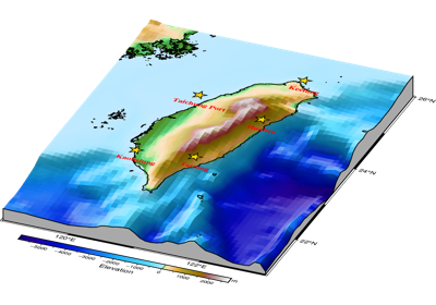
Example
>>> import pygmt
>>> from pygmt.params import Axis, Frame
>>> # Load the 30 arc-minutes grid with "gridline" registration in a given region
>>> grid = pygmt.datasets.load_earth_relief(
...     resolution="30m",
...     region=[-92.5, -82.5, -3, 7],
...     registration="gridline",
... )
>>> # Create a new figure instance with pygmt.Figure()
>>> fig = pygmt.Figure()
>>> # Create the contour plot
>>> fig.grdview(
...     # Pass in the grid downloaded above
...     grid=grid,
...     # Set the perspective to an azimuth of 130° and an elevation of 30°
...     perspective=[130, 30],
...     # Add a frame to the x- and y-axes
...     # Specify annotations on the south and east borders of the plot
...     frame=Frame(axes="wSnE", xaxis=Axis(annot=True), yaxis=Axis(annot=True)),
...     # Set the projection of the 2-D map to Mercator with a 10 cm width
...     projection="M10c",
...     # Set the vertical scale (z-axis) to 2 cm
...     zsize="2c",
...     # Set "surface plot" to color the surface via a CPT
...     surftype="surface",
...     # Specify CPT to "geo"
...     cmap="gmt/geo",
... )
>>> # Show the plot
>>> fig.show()