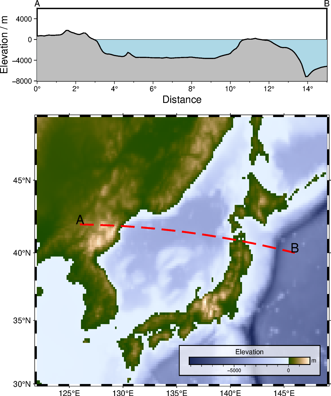
Cross-section along a transect

pygmt.project and pygmt.grdtrack can be used to focus on a quantity and its variation along a desired survey line. In this example, the elevation is extracted from a grid provided via pygmt.datasets.load_earth_relief. The figure consists of two parts, a map of the elevation in the study area showing the survey line and a Cartesian plot showing the elevation along the survey line.

This example is orientated on an example in the GMT/China documentation: https://docs.gmt-china.org/latest/examples/ex026/

import pygmt

# Define region of study area
# lon_min, lon_max, lat_min, lat_max in degrees East and North
region_map = [122, 149, 30, 49]

# Chose a survey line with start point A and end point B
lonA, latA, lonB, latB = 126, 42, 146, 40  # noqa: N816

# Create a new pygmt.Figure instance
fig = pygmt.Figure()

# ----------------------------------------------------------------------------
# Bottom: Map of elevation in study area

# Set up basic map using a Mercator projection with a width of 12 centimeters
fig.basemap(region=region_map, projection="M12c", frame="af")

# Download grid for Earth relief with a resolution of 10 arc-minutes and gridline
# registration [Default]
grid_map = pygmt.datasets.load_earth_relief(resolution="10m", region=region_map)

# Plot the downloaded grid with color-coding based on the elevation
fig.grdimage(grid=grid_map, cmap="oleron")

# Add a colorbar for the elevation
fig.colorbar(
    # Place the colorbar inside the plot (lowercase "j") in the Bottom Right (BR)
    # corner with an offset ("+o") of 0.7 centimeters and 0.3 centimeters in x- or y-
    # directions, respectively; move the x-label above the horizontal colorbar ("+ml")
    position="jBR+o0.7c/0.8c+h+w5c/0.3c+ml",
    # Add a box around the colobar with a fill ("+g") in "white" color and a
    # transparency ("@") of 30 % and with a 0.8-points thick, black, outline ("+p")
    box="+gwhite@30+p0.8p,black",
    # Add x- and y-labels ("+l")
    frame=["x+lElevation", "y+lm"],
)

# Plot the survey line
fig.plot(x=[lonA, lonB], y=[latA, latB], pen="1p,red,solid")

# Add labels "A" and "B" for the start and end points of the survey line
fig.text(
    x=[lonA, lonB],
    y=[latA, latB],
    text=["A", "B"],
    offset="0c/0.3c",  # Move text 0.2 centimeters up (y-direction)
    font="15p,red",  # Use a red font with a size of 15 points
)

# ----------------------------------------------------------------------------
# Top: Elevation along survey line

# Shift plot origin to the top by the height of the map ("+h") plus 1.5 centimeters
fig.shift_origin(yshift="h+1.5c")

fig.basemap(
    region=[0, 15, -8000, 6000],  # x_min, x_max, y_min, y_max
    # Cartesian projection with a width of 12 centimeters and a height of 3 centimeters
    projection="X12c/3c",
    frame=0,
)

# Add labels "A" and "B" for the start and end points of the survey line
fig.text(
    x=[0, 15],
    y=[7000, 7000],
    text=["A", "B"],
    no_clip=True,  # Do not clip text that fall outside the plot bounds
    font="10p,red",
)

# Generate points along a great circle corresponding to the survey line and store them
# in a pandas.DataFrame
track_df = pygmt.project(
    center=[lonA, latA],  # Start point of survey line (longitude, latitude)
    endpoint=[lonB, latB],  # End point of survey line (longitude, latitude)
    generate=0.1,  # Output data in steps of 0.1 degrees
)

# Extract the elevation at the generated points from the downloaded grid and add it as
# new column "elevation" to the pandas.DataFrame
track_df = pygmt.grdtrack(grid=grid_map, points=track_df, newcolname="elevation")

# Plot water masses
fig.plot(
    x=[0, 15],
    y=[0, 0],
    fill="lightblue",  # Fill the polygon in "lightblue"
    pen="0.25p,black,solid",  # Draw a 0.25-points thick, black, solid outline
    close="+y-8000",  # Force closed polygon
)

# Plot elevation along the survey line
fig.plot(
    x=track_df.p,
    y=track_df.elevation,
    fill="gray",
    pen="1p,red,solid",
    close="+y-8000",
)

# Add map frame
# Add annotations ("a") and ticks ("f") as well as labels ("+l") at the west or left
# and south or bottom sides ("WSrt")
fig.basemap(frame=["WSrt", "xa2f1+lDistance+u°", "ya4000+lElevation / m"])

fig.show()