pygmt.Figure.colorbar
- Figure.colorbar(position=None, length=None, width=None, orientation=None, label=None, unit=None, annot=False, tick=False, grid=False, annot_angle=None, annot_prefix=None, annot_unit=None, reverse=False, nan=False, nan_position=None, bg_triangle=False, fg_triangle=False, triangle_height=None, move_text=None, label_as_column=False, box=False, truncate=None, shading=False, log=False, scale=None, monochrome=False, dpi=None, projection=None, region=None, frame=False, verbose=False, panel=False, perspective=False, transparency=None, **kwargs)
Plot gray scale or color scale bar.
Both horizontal and vertical colorbars are supported. For CPTs with gradational colors (i.e., the lower and upper boundary of an interval have different colors) we will interpolate to give a continuous scale. Variations in intensity due to shading/illumination may be displayed by setting the
shadingparameter. Colors may be spaced according to a linear scale, all be equal size, or by providing a file with individual tile widths.Note
For GMT >=6.5.0, the fontsizes of the colorbar x-label, x-annotations, and y-label are scaled based on the width of the colorbar following \(\sqrt{colorbar\_width / 15}\). To set a desired fontsize via the GMT default parameters FONT_ANNOT_PRIMARY, FONT_ANNOT_SECONDARY, and FONT_LABEL (or jointly FONT) users have to divide the desired fontsize by the value calculated with the formula given above before passing it to the default parameters. To only affect fontsizes related to the colorbar, the defaults can be changed locally only using
with pygmt.config(...):.Full GMT docs at https://docs.generic-mapping-tools.org/6.6/colorbar.html.
Aliases:
C = cmap
L = equalsize
Z = zfile
F = box
G = truncate
I = shading
J = projection
M = monochrome
N = dpi
Q = log
R = region
V = verbose
W = scale
c = panel
p = perspective
t = transparency
B = label, unit, annot, tick, grid, annot_angle, annot_prefix, annot_unit
D = position, +w: length/width, +h/+v: orientation, +r: reverse, +n: nan/nan_position, +e: fg_triangle/bg_triangle/triangle_height, +m: move_text/label_as_column
- Parameters:
cmap (str) – File name of a CPT file or a series of comma-separated colors (e.g., color1,color2,color3) to build a linear continuous CPT from those colors automatically.
position (
Position|Sequence[float|str] |Literal['TL','TC','TR','ML','MC','MR','BL','BC','BR'] |None, default:None) –Position of the colorbar on the plot. It can be specified in multiple ways:
A
pygmt.params.Positionobject to fully control the reference point, anchor point, and offset.A sequence of two values representing the x- and y-coordinates in plot coordinates, e.g.,
(1, 2)or("1c", "2c").A 2-character justification code for a position inside the plot, e.g.,
"TL"for Top Left corner inside the plot.
If not specified, defaults to bottom-center outside of the plot.
width (
float|str|None, default:None) – Length and width of the colorbar. If length is given with a unit%then it is in percentage of the corresponding plot side dimension (i.e., plot width for a horizontal colorbar, or plot height for a vertical colorbar). If width is given with unit%then it is in percentage of the bar length. [Length defaults to 80% of the corresponding plot side dimension, and width defaults to 4% of the bar length].unit (
str|None, default:None) – Set the label and unit for the colorbar. The label is placed along the colorbar and the unit is placed at the end of the colorbar.grid (
float|bool, default:False) – Intervals for annotations, ticks, and gridlines. Refer topygmt.params.Axisfor more details on how these parameters work.annot_angle (
float|None, default:None) – The prefix, unit and angle for the annotations. The prefix is placed before the annotation text; the unit is placed after the annotation text; and the angle is the angle of the annotation text.frame (
Frame|Axis|Literal['none'] |str|Sequence[str] |bool, default:False) – Set colorbar boundary frame, labels, and axes attributes. Ifframe=True, a default frame will be drawn. Ifframe="none", no frame will be drawn. Raw GMT strings or sequences of strings are also supported for backward compatibility. For more control over the frame attributes, use parameters such asannot,tick,grid,annot_angle,annot_prefix,annot_unit,label, andunitinstead.orientation (
Literal['horizontal','vertical'] |None, default:None) – Set the colorbar orientation to either"horizontal"or"vertical". [Default is vertical, unlesspositionis set to bottom-center or top-center withcstype="outside"orcstype="inside", then horizontal is the default].reverse (
bool, default:False) – Reverse the positive direction of the bar.nan (
bool, default:False) – Draw a rectangle filled with the NaN color (via the N entry in the CPT or COLOR_NAN if no such entry) at the start or end of the colorbar (controlled vianan_position). If a string is given, use that string as the label for the NaN color.nan_position (
Literal['start','end'] |None, default:None) – Set the position of the NaN rectangle. Choose either"start"or"end"to place the NaN color rectangle at the start or end of the colorbar [Default is"start"].bg_triangle (
bool, default:False)fg_triangle (
bool, default:False) – IfTrue, draw triangles for the back- or foreground colors [Default is no triangles]. The back- and/or foreground colors are taken from the B and F entries in the CPT. If no such entries exist, then the system default colors for B and F are used instead (COLOR_BACKGROUND and COLOR_FOREGROUND).triangle_height (
float|None, default:None) – Height of the triangles for back- and foreground colors [Default is half of the bar width].move_text (
Literal['annotations','label','unit'] |Sequence[str] |None, default:None) – Move text (annotations, label, and unit) to opposite side. Accept a sequence of strings containing one or more of"annotations","label", and"unit". The default placements of these texts depend on the colorbar orientation and position.label_as_column (
bool, default:False) – Print a vertical label as a column of characters (does not work with special characters).box (
Box|bool, default:False) – Draw a background box behind the colorbar. If set toTrue, a simple rectangular box is drawn using MAP_FRAME_PEN. To customize the box appearance, pass apygmt.params.Boxobject to control style, fill, pen, and other box properties.truncate (
Sequence[float] |None, default:None) – (zlow, zhigh). Truncate the incoming CPT so that the lowest and highest z-levels are to zlow and zhigh. If one of these equal NaN then we leave that end of the CPT alone. The truncation takes place before the plotting.scale (
float|None, default:None) – Multiply all z-values in the CPT by the provided scale. By default, the CPT is used as is.shading (
float|Sequence[float] |bool, default:False) –Add illumination effects [Default is no illumination].
If
True, a default intensity range of -1 to +1 is used.Passing a single numerical value max_intens sets the range of intensities from -max_intens to +max_intens.
Passing a sequence of two numerical values (low, high) sets the intensity range from low to high to specify an asymmetric range.
equalsize (float or str) – [i][gap]. Equal-sized color rectangles. By default, the rectangles are scaled according to the z-range in the CPT (see also
zfile). If gap is appended and the CPT is discrete each annotation is centered on each rectangle, using the lower boundary z-value for the annotation. If i is prepended the interval range is annotated instead. Ifshadingis used each rectangle will have its constant color modified by the specified intensity.log (
bool, default:False) – Select logarithmic scale and power of ten annotations. All z-values in the CPT will be converted to \(p = \log_{10}(z)\) and only integer p values will be annotated using the \(10^{p}\) format [Default is linear scale].zfile (str) – File with colorbar-width per color entry. By default, the width of the entry is scaled to the color range, i.e., z = 0-100 gives twice the width as z = 100-150 (see also
equalsize). Note: The widths may be in plot distance units or given as relative fractions and will be automatically scaled so that the sum of the widths equals the requested colorbar length.monochrome (
bool, default:False) – Force a monochrome graybar using the (television) YIQ transformation.dpi (
int|None, default:None) –Control how the color scale should be encoded graphically.
Use a positive integer to draw the color scale as image and set the effective dots-per-inch for rasterization of color scales, which is useful for continuous colormaps.
Use
dpi=0to draw color rectangles, which is useful for discrete colormaps.
If not specified, GMT uses its default encoding behavior, and the default dpi is 600 if the colorbar is drawn as image.
projection (
str|None, default:None) – projcode[projparams/]width|scale. Select map projection.region (str or list) – xmin/xmax/ymin/ymax[+r][+uunit]. Specify the region of interest.
verbose (bool or str) – Select verbosity level [Full usage].
panel (
int|Sequence[int] |bool, default:False) –Select a specific subplot panel. Only allowed when used in
Figure.subplotmode.Trueto advance to the next panel in the selected order.index to specify the index of the desired panel.
(row, col) to specify the row and column of the desired panel.
The panel order is determined by the
Figure.subplotmethod. row, col and index all start at 0.perspective (
float|Sequence[float] |str|bool, default:False) –Select perspective view and set the azimuth and elevation of the viewpoint.
Accepts a single value or a sequence of two or three values: azimuth, (azimuth, elevation), or (azimuth, elevation, zlevel).
azimuth: Azimuth angle of the viewpoint in degrees [Default is 180, i.e., looking from south to north].
elevation: Elevation angle of the viewpoint above the horizon [Default is 90, i.e., looking straight down at nadir].
zlevel: Z-level at which 2-D elements (e.g., the plot frame) are drawn. Only applied when used together with
zsizeorzscale. [Default is at the bottom of the z-axis].
Alternatively, set
perspective=Trueto reuse the perspective setting from the previous plotting method, or pass a string following the full GMT syntax for finer control (e.g., adding+wor+vmodifiers to select an axis location other than the plot origin). See https://docs.generic-mapping-tools.org/6.6/gmt.html#perspective-full for details.transparency (float) – Set transparency level, in [0-100] percent range [Default is
0, i.e., opaque]. Only visible when PDF or raster format output is selected. Only the PNG format selection adds a transparency layer in the image (for further processing).
Example
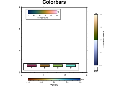
>>> import pygmt
>>> # Create a new figure instance with pygmt.Figure()
>>> fig = pygmt.Figure()
>>> # Create a basemap
>>> fig.basemap(region=[0, 10, 0, 3], projection="X10c/3c", frame=True)
>>> # Call the colorbar method for the plot
>>> fig.colorbar(cmap="SCM/roma", label="Velocity", unit="m/s")
>>> # Show the plot
>>> fig.show()
Examples using pygmt.Figure.colorbar
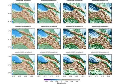
Calculating grid gradient with custom azimuth and normalization parameters