Note
Go to the end to download the full example code.
2. Create a contour map
This tutorial page covers the basics of creating a figure of the Earth relief, using a
remote dataset hosted by GMT, using the method pygmt.datasets.load_earth_relief.
It will use the pygmt.Figure.grdimage, pygmt.Figure.grdcontour,
pygmt.Figure.colorbar, and pygmt.Figure.coast methods for plotting.
import pygmt
Loading the Earth relief dataset
The first step is to use pygmt.datasets.load_earth_relief. The resolution
parameter sets the resolution of the remote grid file, which will affect the
resolution of the plot made later in the tutorial. The registration parameter
determines the grid registration.
This grid region covers the islands of Guam and Rota in the western Pacific Ocean.
grid = pygmt.datasets.load_earth_relief(
    resolution="30s", region=[144.5, 145.5, 13, 14.5], registration="gridline"
)
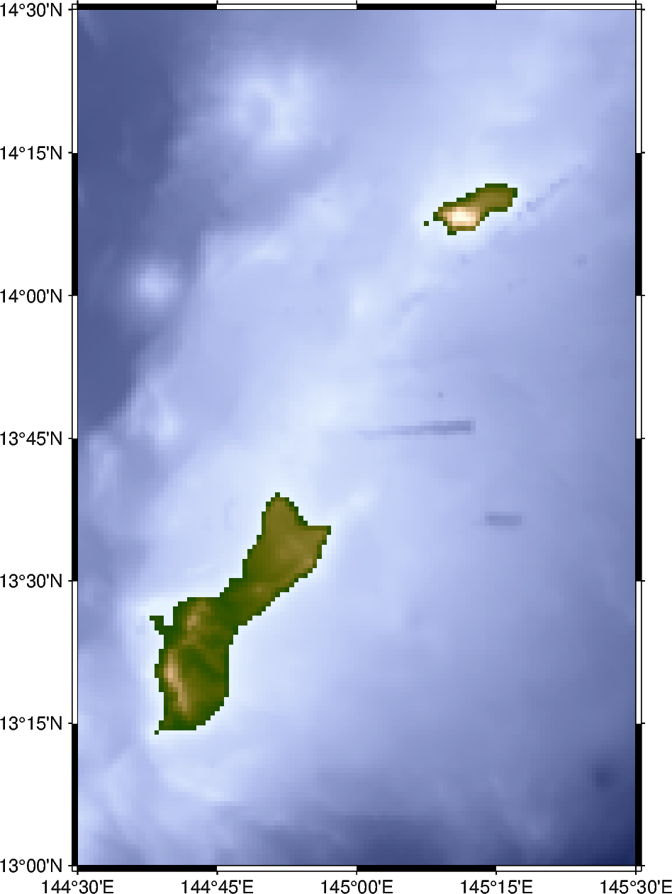
Plotting Earth relief
To plot Earth relief data, the method pygmt.Figure.grdimage can be used to
plot a color-coded figure to display the topography and bathymetry in the grid file.
The grid parameter accepts the input grid, which in this case is the remote file
downloaded in the previous step. If the region parameter is not set, the region
boundaries of the input grid are used.
The cmap parameter sets the color palette table (CPT) used for portraying the
Earth relief. The pygmt.Figure.grdimage method uses the input grid to relate
the Earth relief values to a specific color within the CPT. In this case, the CPT
“oleron” is used; a full list of CPTs can be found at https://docs.generic-mapping-tools.org/6.5/reference/cpts.html.
fig = pygmt.Figure()
fig.grdimage(grid=grid, frame="a", projection="M10c", cmap="oleron")
fig.show()
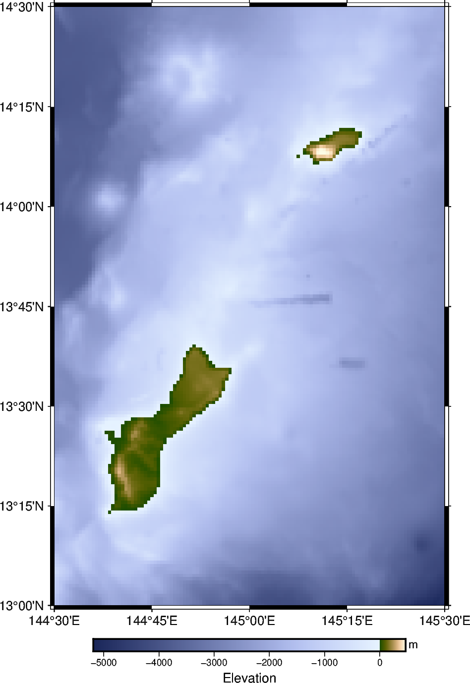
Adding a colorbar
To show how the plotted colors relate to the Earth relief, a colorbar can be added
using the pygmt.Figure.colorbar method.
To control the annotation and labels on the colorbar, a list is passed to the
frame parameter. The value beginning with "a" sets the interval for the
annotation on the colorbar, in this case every 1,000 meters. To set the label for an
axis on the colorbar, the argument begins with either "x+l" (x-axis) or "y+l"
(y-axis), followed by the intended label.
By default, the CPT for the colorbar is the same as the one set in
pygmt.Figure.grdimage.
fig = pygmt.Figure()
fig.grdimage(grid=grid, frame="a", projection="M10c", cmap="oleron")
fig.colorbar(frame=["a1000", "x+lElevation", "y+lm"])
fig.show()
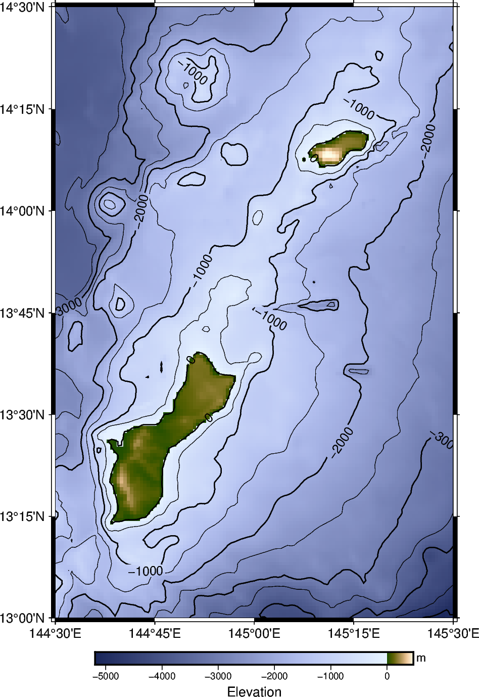
Adding contour lines
To add contour lines to the color-coded figure, the pygmt.Figure.grdcontour
method is used. The frame and projection are already set using
pygmt.Figure.grdimage and are not needed again. However, the same input for
grid (in this case, the variable named “grid”) must be input again. The levels
parameter sets the spacing between adjacent contour lines (in this case, 500 meters).
The annotation parameter annotates the contour lines corresponding to the given
interval (in this case, 1,000 meters) with the related values, here elevation or
bathymetry. By default, these contour lines are drawn thicker. Optionally, the
appearance (thickness, color, style) of the annotated and the not-annotated contour
lines can be adjusted (separately) by specifying the desired pen.
fig = pygmt.Figure()
fig.grdimage(grid=grid, frame="a", projection="M10c", cmap="oleron")
fig.grdcontour(grid=grid, levels=500, annotation=1000)
fig.colorbar(frame=["a1000", "x+lElevation", "y+lm"])
fig.show()
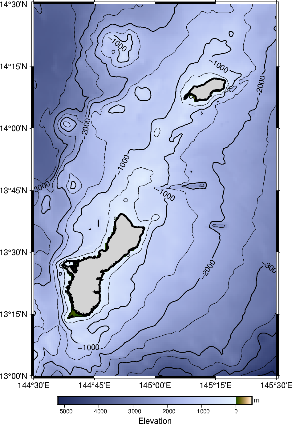
Color in land
To make it clear where the islands are located, the pygmt.Figure.coast method
can be used to color in the landmasses. The land is colored in as “lightgray”, and
the shorelines parameter draws a border around the islands.
fig = pygmt.Figure()
fig.grdimage(grid=grid, frame="a", projection="M10c", cmap="oleron")
fig.grdcontour(grid=grid, levels=500, annotation=1000)
fig.coast(shorelines="2p", land="lightgray")
fig.colorbar(frame=["a1000", "x+lElevation", "y+lm"])
fig.show()
Additional exercises
This is the end of the second tutorial. Here are some additional exercises for the concepts that were discussed:
Change the resolution of the grid file to either
"01m"(1 arc-minute, a lower resolution) or"15s"(15 arc-seconds, a higher resolution). Note that higher resolution grids will have larger file sizes. Available resolutions can be found atpygmt.datasets.load_earth_relief.Create a contour map of the area around Mt. Rainier. A suggestion for the
regionwould be[-122, -121, 46.5, 47.5]. Adjust thepygmt.Figure.grdcontourandpygmt.Figure.colorbarsettings as needed to make the figure look good.Create a contour map of São Miguel Island in the Azores; a suggested
regionis[-26, -25, 37.5, 38]. Instead of coloring inland, setwaterto “lightblue” to only display Earth relief information for the land.Try other CPTs, such as “SCM/fes” or “geo”.
Total running time of the script: (0 minutes 0.978 seconds)