pygmt.Figure.coast
- Figure.coast(resolution=None, land=None, water=None, rivers=None, borders=None, shorelines=False, map_scale=None, box=False, projection=None, region=None, frame=False, verbose=False, panel=False, perspective=False, transparency=None, **kwargs)
Plot continents, countries, shorelines, rivers, and borders.
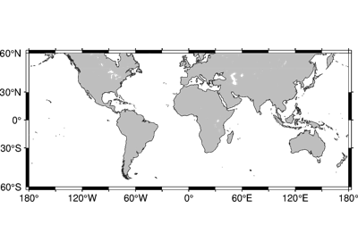
Plots grayshaded, colored, or textured land masses [or water masses] on maps and [optionally] draws coastlines, rivers, and political boundaries. The data files come in 5 different resolutions: (f)ull, (h)igh, (i)ntermediate, (l)ow, and (c)rude. The full resolution files amount to more than 55 Mb of data and provide great detail; for maps of larger geographical extent it is more economical to use one of the other resolutions. If the user selects to paint the land areas and does not specify fill of water areas then the latter will be transparent (i.e., earlier graphics drawn in those areas will not be overwritten). Likewise, if the water areas are painted and no land fill is set then the land areas will be transparent.
A map projection must be supplied.
Full GMT docs at https://docs.generic-mapping-tools.org/6.6/coast.html.
Aliases:
A = area_thresh
C = lakes
E = dcw
B = frame
D = resolution
F = box
G = land
I = rivers
J = projection
L = map_scale
R = region
S = water
V = verbose
c = panel
p = perspective
t = transparency
- Parameters:
area_thresh (float or str) – min_area[/min_level/max_level][+a[g|i][s|S]][+l|r][+ppercent]. Features with an area smaller than min_area in km2 or of hierarchical level that is lower than min_level or higher than max_level will not be plotted [Default is
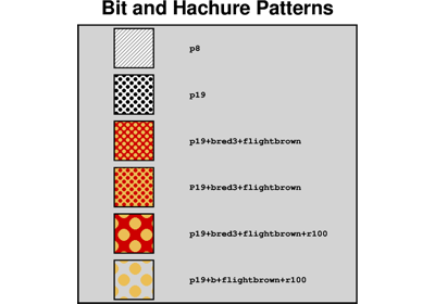
"0/0/4"(all features)].lakes (str or list) – fill[+l|+r]. Set the shade, color, or pattern for lakes and river-lakes. The default is the fill chosen for “wet” areas set by the
waterparameter. Optionally, specify separate fills by appending +l for lakes or +r for river-lakes, and passing multiple strings in a list.resolution (
Literal['auto','full','high','intermediate','low','crude',None], default:None) – Select the resolution of the coastline dataset to use. The available resolutions from highest to lowest are:"full","high","intermediate","low", and"crude", which drops by 80% between levels. Default is"auto"to automatically select the most suitable resolution given the chosen map scale.land (
str|None, default:None) – Select filling of “dry” areas.water (
str|None, default:None) – Select filling of “wet” areas.rivers (
int|str|Sequence[int|str] |None, default:None) –Draw rivers. Specify the type of rivers to draw, and optionally append a pen attribute, in the format river/pen [Default pen is
"0.25p,black,solid"]. Pass a sequence of river types or river/pen strings to draw different river types with different pens.Choose from the following river types:
0: Double-lined rivers (river-lakes)1: Permanent major rivers2: Additional major rivers3: Additional rivers4: Minor rivers5: Intermittent rivers - major6: Intermittent rivers - additional7: Intermittent rivers - minor8: Major canals9: Minor canals10: Irrigation canals
Or choose from the following preconfigured river groups:
"a": All rivers and canals (types0-10)"A": Rivers and canals except river-lakes (types1-10)"r": Permanent rivers (types0-4)"R": Permanent rivers except river-lakes (types1-4)"i": Intermittent rivers (types5-7)"c": Canals (types8-10)
Example usage:
rivers=1: Draw permanent major rivers with default pen.rivers="1/0.5p,blue": Draw permanent major rivers with a 0.5-point blue pen.rivers=["1/0.5p,blue", "5/0.3p,cyan,dashed"]: Draw permanent major rivers with a 0.5-point blue pen and intermittent major rivers with a 0.3-point dashed cyan pen.
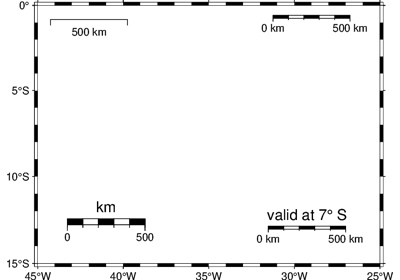
map_scale (
str|None, default:None) –Draw a map scale bar on the plot.
Deprecated since version v0.19.0: Use
pygmt.Figure.scalebarinstead. This parameter is maintained for backward compatibility and accepts raw GMT CLI strings for the-Loption.box (
Box|bool, default:False) – Draw a background box behind the map scale or rose. If set toTrue, a simple rectangular box is drawn using MAP_FRAME_PEN. To customize the box appearance, pass apygmt.params.Boxobject to control style, fill, pen, and other box properties.borders (
int|str|Sequence[int|str] |None, default:None) –Draw political boundaries. Specify the type of boundary to draw, and optionally append a pen attribute, in the format border/pen [Default pen is
"0.25p,black,solid"]. Pass a sequence of border types or border/pen strings to draw different border types with different pens.Choose from the following border types:
1: National boundaries2: State boundaries within the Americas3: Marine boundaries"a": All boundaries (types1-3)
Example usage:
borders=1: Draw national boundaries with default pen.borders="1/0.5p,red": Draw national boundaries with a 0.5-point red pen.borders=["1/0.5p,red", "2/0.3p,blue,dashed"]: Draw national boundaries with a 0.5-point red pen and state boundaries with a 0.3-point dashed blue pen.
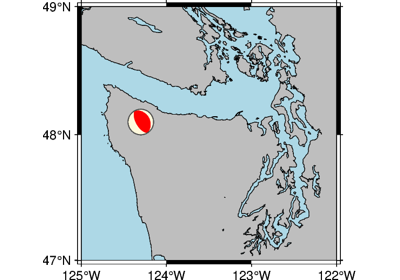
shorelines (
bool|str|Sequence[int|str], default:False) –Draw shorelines. Specify the pen attributes for shorelines [Default pen is
"0.25p,black,solid"]. Shorelines have four levels; by default, the same pen is used for all levels. To specify the shoreline level, use the format level/pen. Pass a sequence of level/pen strings to draw different shoreline levels with different pens. When specific level pens are set, those not listed will not be drawn [Default draws all levels].shorelines=Truedraws all levels with the default pen.Choose from the following shoreline levels:
1: Coastline2: Lakeshore3: Island-in-lake shore4: Lake-in-island-in-lake shore
Example usage:
shorelines=True: Draw all shoreline levels with default pen.shorelines="0.5p,blue": Draw all shoreline levels with a 0.5-point blue pen.shorelines="1/0.5p,black": Draw only coastlines with a 0.5-point black pen.shorelines=["1/0.8p,black", "2/0.4p,blue"]: Draw coastlines with a 0.8-point black pen and lakeshores with a 0.4-point blue pen.
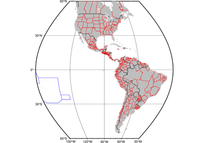
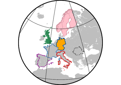
dcw (str or list) – code1,code2,…[+gfill][+ppen][+z]. Select painting country polygons from the Digital Chart of the World. Append one or more comma-separated countries using the 2-letter ISO 3166-1 alpha-2 convention. To select a state of a country (if available), append .state, (e.g,
"US.TX"for Texas). To specify a whole continent, prepend = to any of the continent codes (e.g."=EU"for Europe). Append +ppen to draw polygon outlines [Default is no outline] and +gfill to fill them [Default is no fill].projection (
str|None, default:None) – projcode[projparams/]width|scale. Select map projection.region (str or list) – xmin/xmax/ymin/ymax[+r][+uunit]. Specify the region of interest. Required if this is the first plot command.
frame (
Frame|Axis|Literal['none'] |str|Sequence[str] |bool, default:False) – Set frame and axes attributes for the plot. It can be a bool,"none", apygmt.params.Frameorpygmt.params.Axisobject. Raw GMT strings or sequences of strings are also supported for backward compatibility. Ifframe=True, the frame will be drawn with the default attributes. Ifframe="none", no frame will be drawn. Use apygmt.params.Frameorpygmt.params.Axisobject for more control over the attributes of the frame and axes. A tutorial is available at frame and axes attributes. Full documentation is at https://docs.generic-mapping-tools.org/6.6/gmt.html#b-full.verbose (bool or str) – Select verbosity level [Full usage].
panel (
int|Sequence[int] |bool, default:False) –Select a specific subplot panel. Only allowed when used in
Figure.subplotmode.Trueto advance to the next panel in the selected order.index to specify the index of the desired panel.
(row, col) to specify the row and column of the desired panel.
The panel order is determined by the
Figure.subplotmethod. row, col and index all start at 0.perspective (
float|Sequence[float] |str|bool, default:False) –Select perspective view and set the azimuth and elevation of the viewpoint.
Accepts a single value or a sequence of two or three values: azimuth, (azimuth, elevation), or (azimuth, elevation, zlevel).
azimuth: Azimuth angle of the viewpoint in degrees [Default is 180, i.e., looking from south to north].
elevation: Elevation angle of the viewpoint above the horizon [Default is 90, i.e., looking straight down at nadir].
zlevel: Z-level at which 2-D elements (e.g., the plot frame) are drawn. Only applied when used together with
zsizeorzscale. [Default is at the bottom of the z-axis].
Alternatively, set
perspective=Trueto reuse the perspective setting from the previous plotting method, or pass a string following the full GMT syntax for finer control (e.g., adding+wor+vmodifiers to select an axis location other than the plot origin). See https://docs.generic-mapping-tools.org/6.6/gmt.html#perspective-full for details.transparency (float) – Set transparency level, in [0-100] percent range [Default is
0, i.e., opaque]. Only visible when PDF or raster format output is selected. Only the PNG format selection adds a transparency layer in the image (for further processing).
See also
pygmt.Figure.directional_roseAdd a map directional rose.
pygmt.Figure.magnetic_roseAdd a map magnetic rose.
pygmt.Figure.scalebarAdd a scale bar.
Example
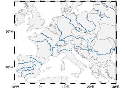
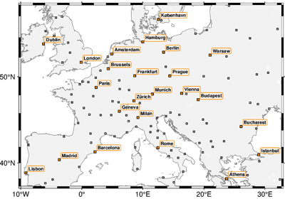
>>> import pygmt
>>> from pygmt.params import Axis
>>> # Create a new plot with pygmt.Figure()
>>> fig = pygmt.Figure()
>>> # Call the coast method for the plot
>>> fig.coast(
...     # Set the projection to Mercator, and the plot width to 10 centimeters
...     projection="M10c",
...     # Set the region of the plot
...     region=[-10, 30, 30, 60],
...     # Set the frame of the plot, here annotations and major ticks
...     frame=Axis(annot=True),
...     # Set the color of the land to "darkgreen"
...     land="darkgreen",
...     # Set the color of the water to "lightblue"
...     water="lightblue",
...     # Draw national borders with a 1-point black line
...     borders="1/1p,black",
... )
>>> # Show the plot
>>> fig.show()
Examples using pygmt.Figure.coast
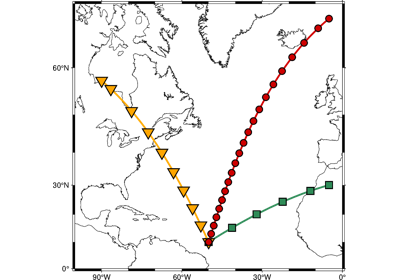
GeoPandas: Plotting lines with LineString or MultiLineString geometry


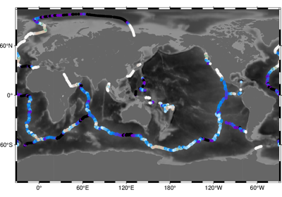
GeoPandas: Plotting points with Point or MultiPoint geometry