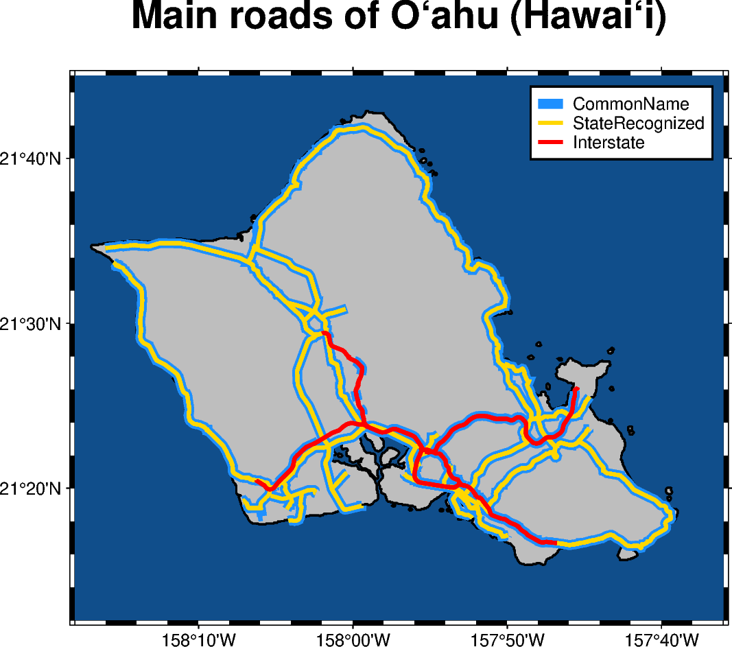
Roads

The pygmt.Figure.plot method allows us to plot geographical data such as lines which are stored in a geopandas.GeoDataFrame object. Use geopandas.read_file to load data from any supported OGR format such as a shapefile (.shp), GeoJSON (.geojson), geopackage (.gpkg), etc. Then, pass the geopandas.GeoDataFrame as an argument to the data parameter of pygmt.Figure.plot, and style the geometry using the pen parameter.

import geopandas as gpd
import pygmt

# Read shapefile data using geopandas
gdf = gpd.read_file(
    "https://www2.census.gov/geo/tiger/TIGER2015/PRISECROADS/tl_2015_15_prisecroads.zip"
)
# The dataset contains different road types listed in the RTTYP column,
# here we select the following ones to plot:
roads_common = gdf[gdf.RTTYP == "M"]  # Common name roads
roads_state = gdf[gdf.RTTYP == "S"]  # State recognized roads
roads_interstate = gdf[gdf.RTTYP == "I"]  # Interstate roads

fig = pygmt.Figure()

# Define target region around Oʻahu (Hawaiʻi)
region = [-158.3, -157.6, 21.2, 21.75]  # xmin, xmax, ymin, ymax

title = "Main roads of O`ahu (Hawai`i)"  # Approximating the Okina letter ʻ with `
fig.basemap(region=region, projection="M12c", frame=["af", f"WSne+t{title}"])
fig.coast(land="gray", water="dodgerblue4", shorelines="1p,black")

# Plot the individual road types with different pen settings and assign labels
# which are displayed in the legend
fig.plot(data=roads_common, pen="5p,dodgerblue", label="CommonName")
fig.plot(data=roads_state, pen="2p,gold", label="StateRecognized")
fig.plot(data=roads_interstate, pen="2p,red", label="Interstate")

# Add legend
fig.legend()

fig.show()